Dyson sphere design and construction

Overview

The following guide describes information regarding both basic dyson sphere design, basic construction information as well as technical data regarding design of a dyson sphere. Anyone interested in technical aspects of the design may find something of use in this guide.

Preamble and disclaimers

#1 – All data in this guide is compiled from experimental data;

#2 – All data, is compiled in version 0.6.15.5655; As Dyson Sphere Program is an early access game exact values may change without notice. Any and all values are calculated from that specific version alone. Data was used last time in version 0.6.15.5678 revision.

#3 – [direct result of #1] – due to data being compiled from in-game data, and due to fact that numbers in-game are rounded down, the values provided may not be exact. Example of prediction does have discrepancy between actual and expected values, though the degree of difference is quite low, and may be either due to an error in the calculation or case of code-based rounding in calculation.

#4 – due to data being compiled experimentally any correction is welcome, with the assumption that said correction improves accuracy of prediction.

#5 – all comparison data in dedicated specification sections are all made using default Dyson shell – that is 10 000 radius, 0 inclination and 0 longitude.

#6 – please remember that all pictures/screenshots can be clicked on for higher size/quality of an image.

NOTE: Solar Sails have limited lifetime and 36 kW generation at luminosity 1.000 star. Integration process changes them into Cell points, with unlimited lifetime and 15 kW generation at luminosity 1.000 star. Please keep that in mind.
In the guide whenever ‘Solar Sail’ is mentioned a solar sail item or a solar sail in a Dyson swarm is implied.
Whenever ‘Cell point’ is mentioned a solar cell integrated into Dyson sphere (and listed in the node as ‘cell point’ is implied.

Table of contents

The following parts are in regards to the Dyson spheres in this guide:

– Dyson Sphere Construction Basics – this section describes basic information ‘how to build any Dyson Sphere, what one needs to do, and how to do it’. This part is best skipped by those who are looking for design and implication, and know both how to build a sphere and fill its’ cell points, but has at least 1 mechanics that may not be immediately obvious, even to those who built sphere already.

– Power Production model – quick description of in-game power production model of a Dyson Sphere.
– Case Study [Predictive capability and accuracy] – examples of calculation of power production of a Dyson Sphere, using power production model, these are used as examples that model has predictive capability, but is not perfect.
– Link type effect – quick note regarding link types used in design;
– Sphere construction cost – basic information regarding cost calculation of a Dyson Sphere’s structure.

– Design Implications – Implications from power production model and construction cost model. Also includes example designs]. For TL:DR version go there.

– Power Density Dyson Sphere – technical comparison data of sphere created with power density in mind; Cost efficiency be damned [see design implication], this is how to pump as much power from a sphere as possible. Currently most power dense design that I know of. If you find better design – let me know.
– Cost Efficiency Dyson Sphere – technical comparison data of sphere created with cost efficiency in mind; Power density be damned [see design implication], this is how to get as much energy from your star as possible with lowest cost. Currently most cost efficient design I know. If you find better design – let me know.
– ‘Football’ Design Dyson Sphere – technical comparison data of a ‘football design’ a Dyson sphere with a step-by-step guide how to design it. While sub-optimal for cost efficiency, and bad for power density it has some degree of regularity and aesthetics.

– Energy Retrieval from the Dyson System – Basic – this part speaks about requirements regarding taking energy from the system, how graviton lenses affect power production and how energy is distributed between receivers, if the Dyson System cannot fill the demand.
– Energy Retrieval from the Dyson System – Implications – this part talks about 3 implications from information covered beforehand in this guide, when it comes to ray receivers. Not all of them are obvious.

Dyson Sphere Construction Basics [version 1]

There are 3 general stages of construction of a Dyson Sphere.

Design is quite generalized and extremely fluid; Few design considerations are what most of this guide is about, together with few design examples, as such only basic how to is mentioned in this guide, including what to keep in mind.

What may not be immediately obvious is that Dyson Sphere design capability is unlocked with solar sail technology:

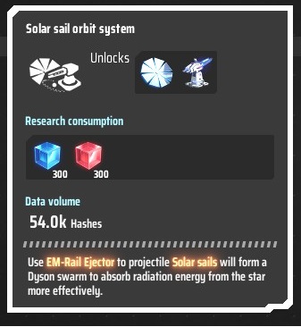
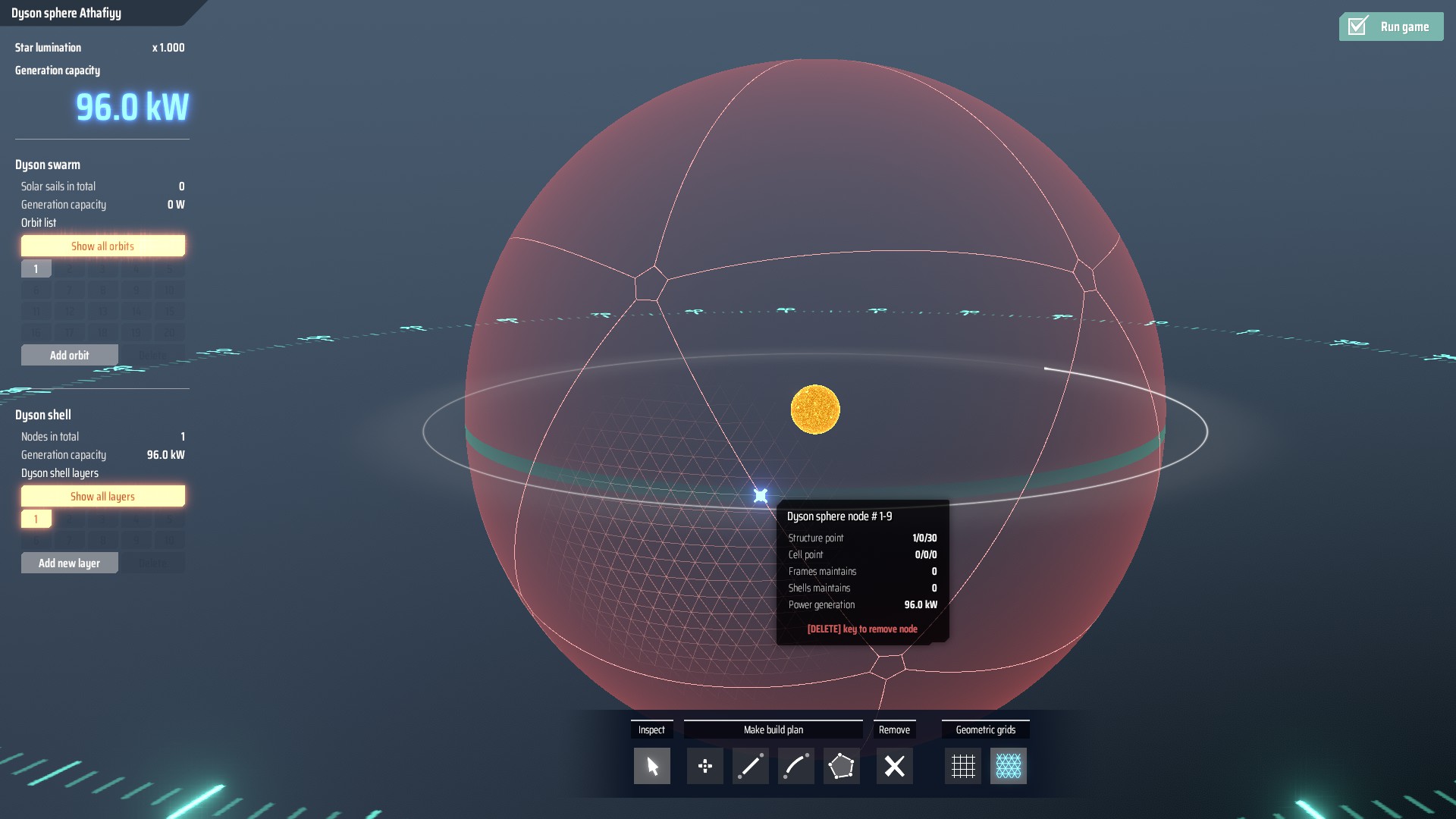
With this technology Dyson sphere design window is available, and a default shell and default sphere areas are defined.

Default solar sail orbit data:

Default dyson shell data:

For basic purposes one can use those existing elements for purposes of design and construction.

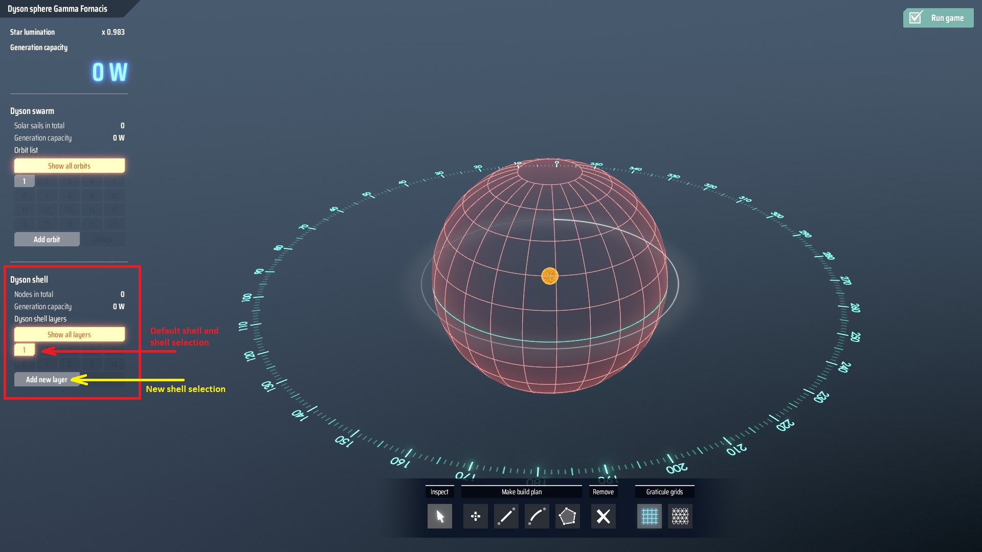
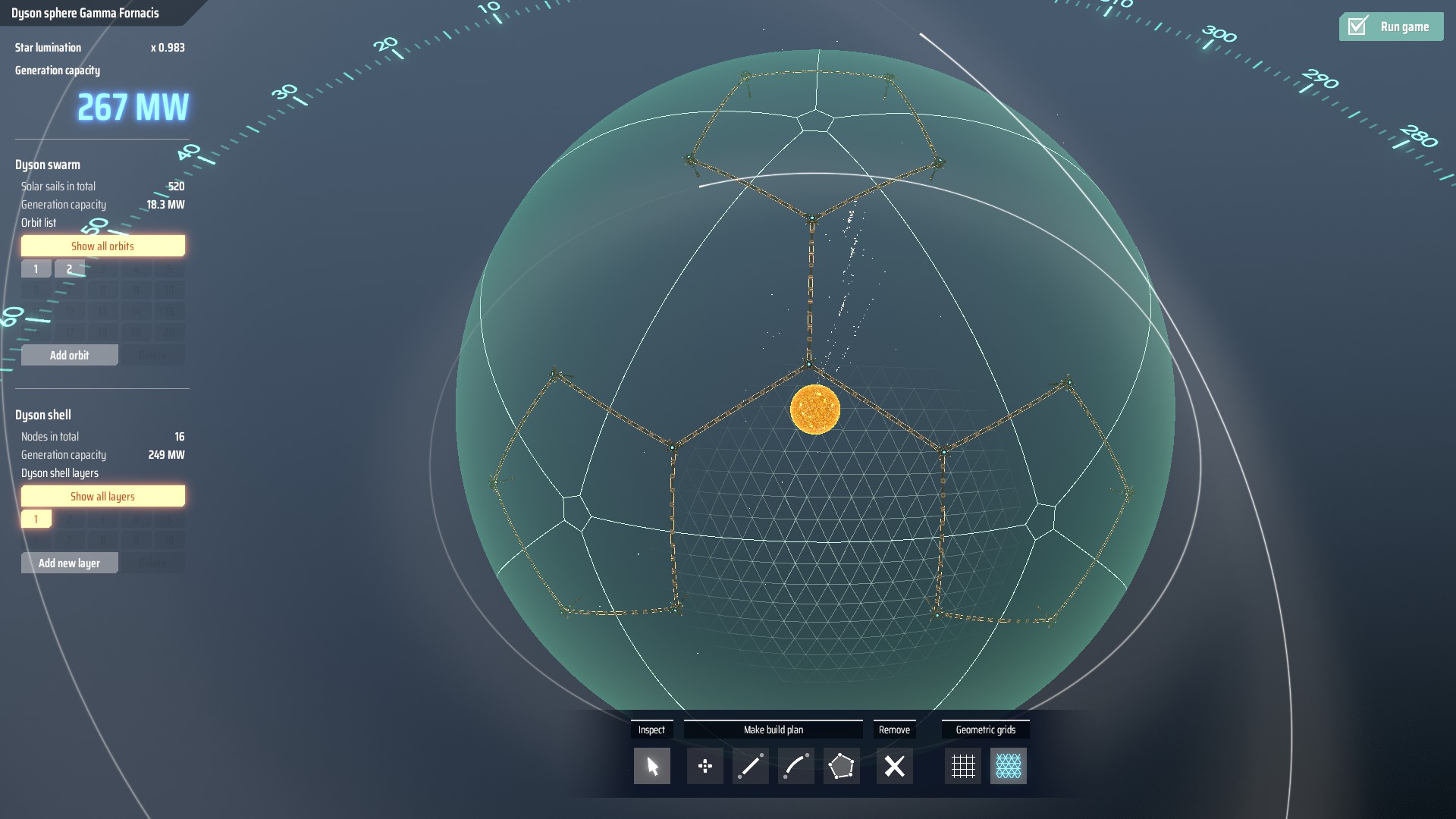
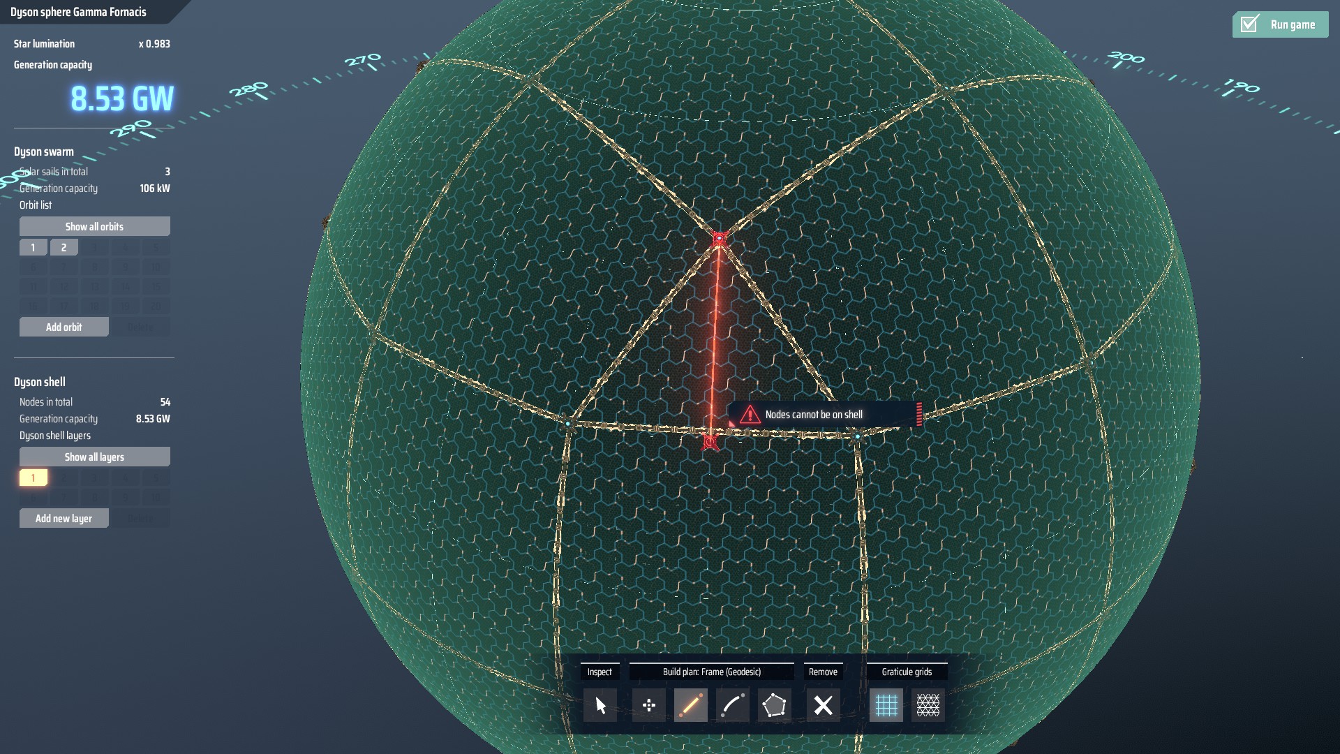
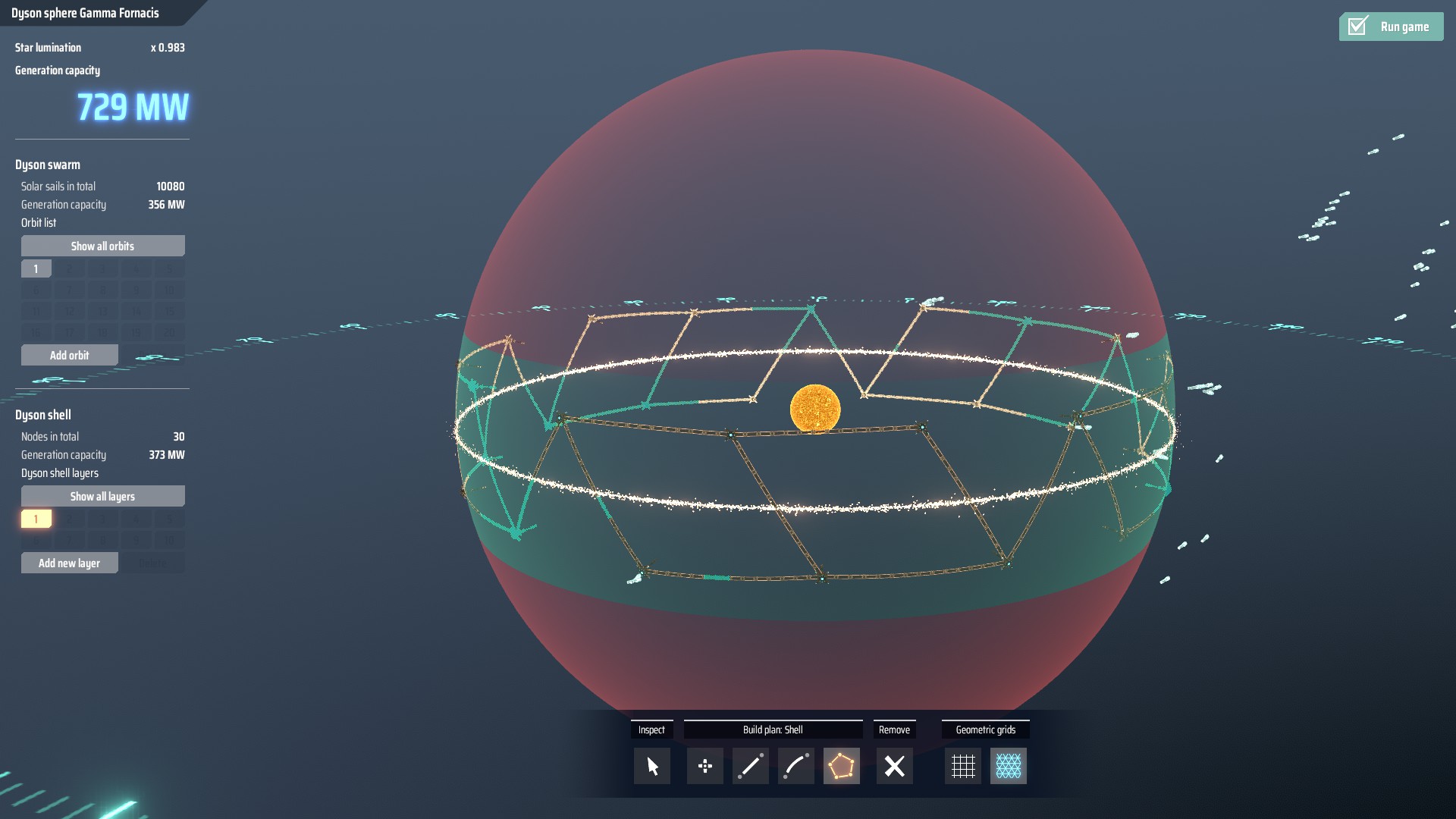
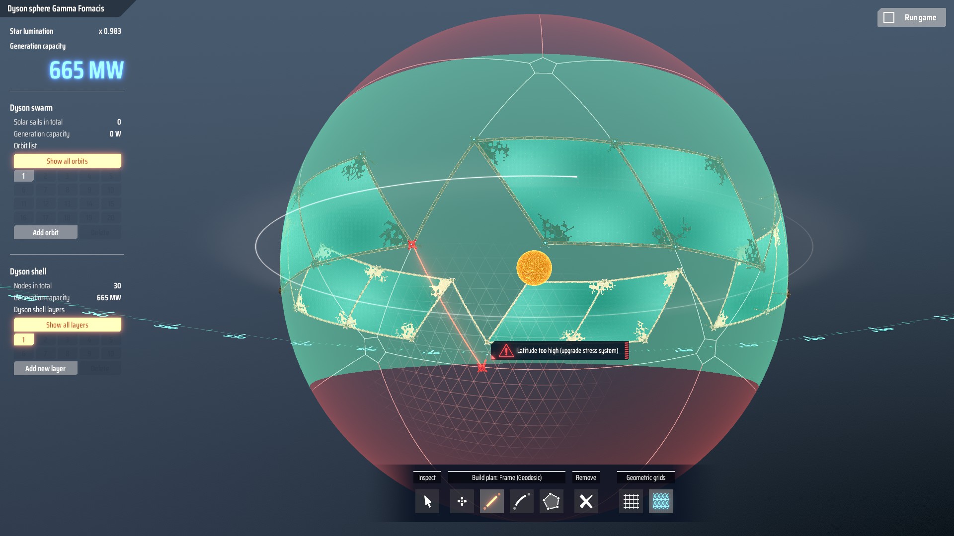
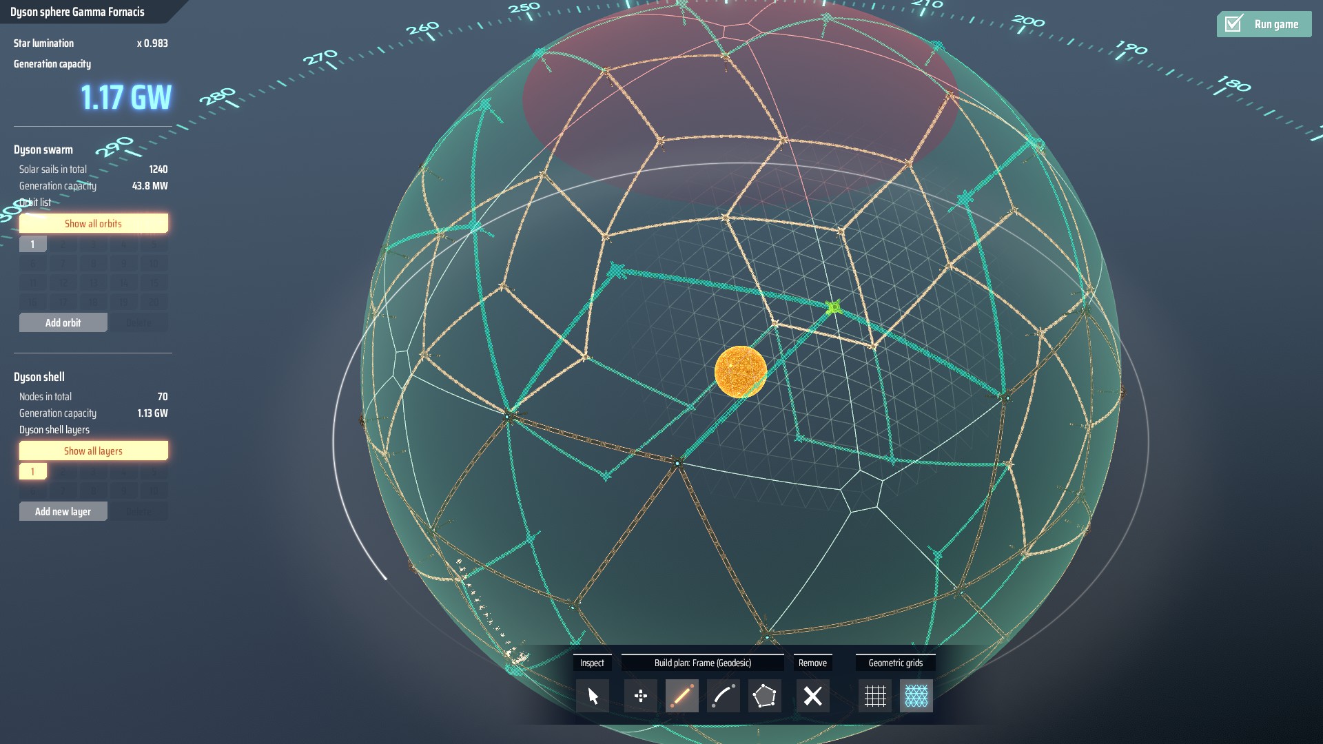
First step to design of a Dyson Sphere is a selection of a shell [own shell can be made using ‘add layer’ option below the list of Dyson shells, as shown below. The shell will be shown in [most likely] mostly red outline, as shown above.

The red and teal [I hope that’s how that color is officially called; correct me if I’m wrong], show respectively areas that we cannot build in, and areas that we can build in using current Dyson Sphere Structural System research level. as shown below

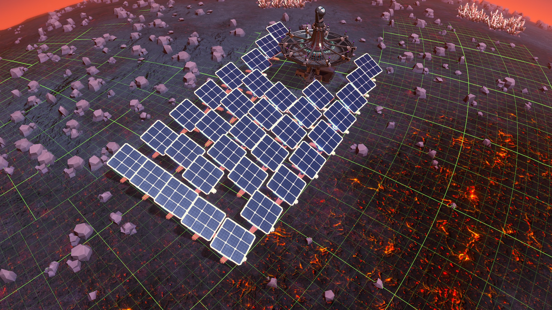
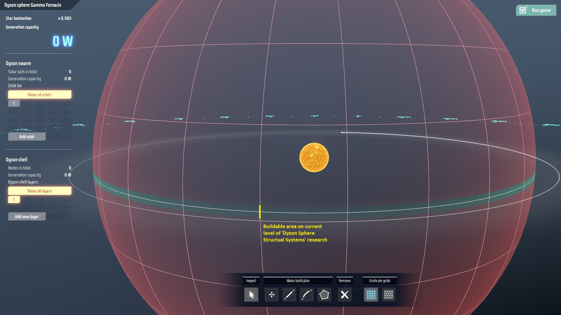It should be noted that default grid – Graticule grid as it is known, is relatively good estimation of research level needed to build in specific area:

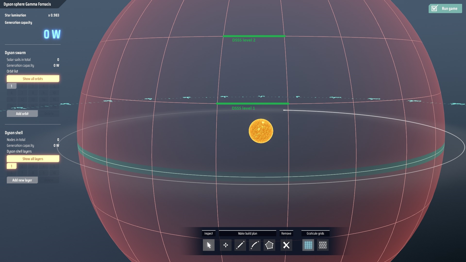
While the line of buildable area will be slightly further than that, the nodes will generally be placed up to those thicker lines on the graticule grid.

The following options allow us to design a sphere: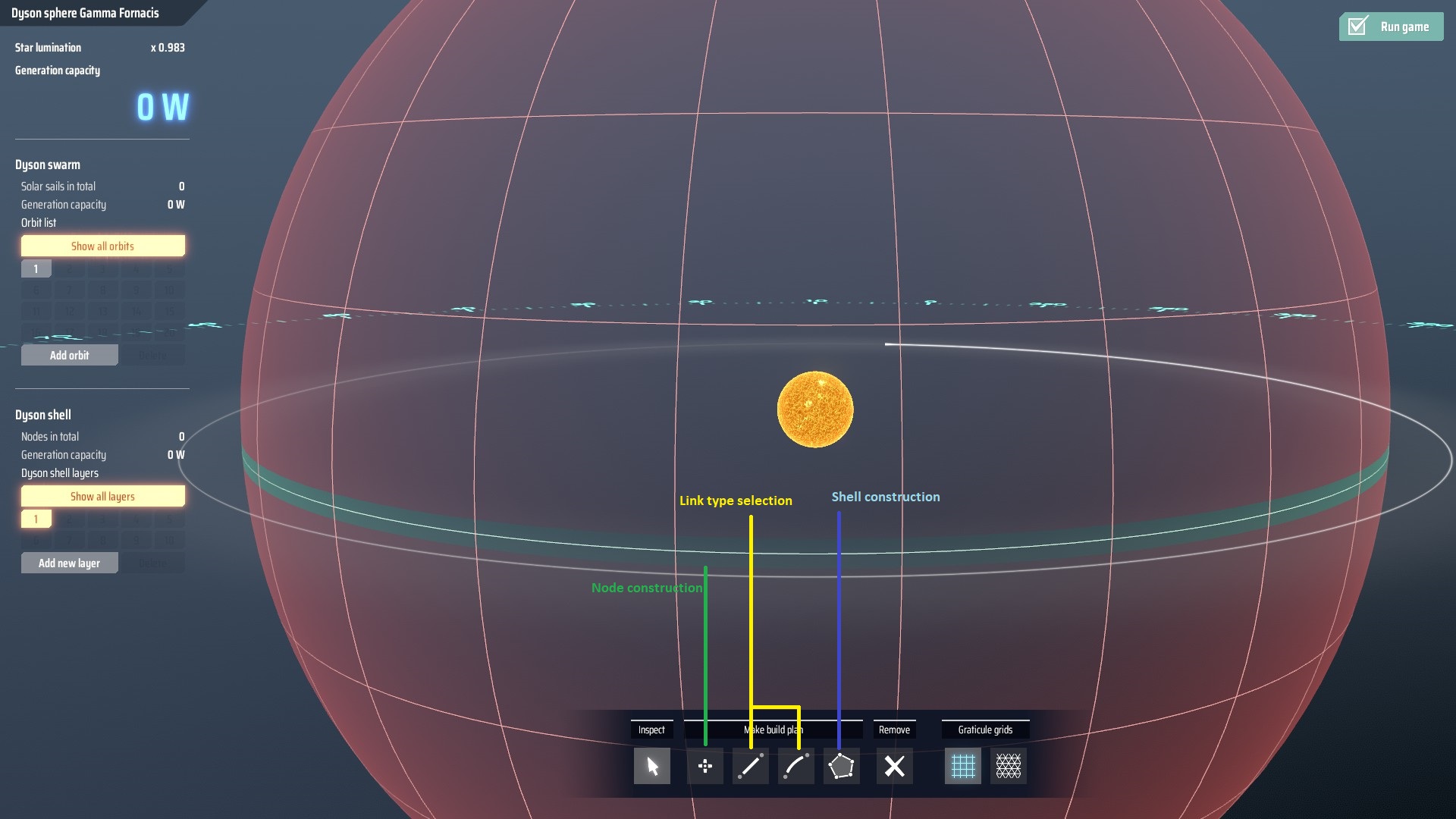

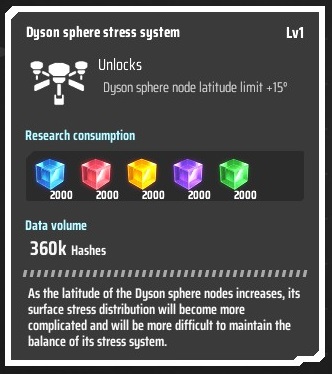
Node mode allows us to place a single nodes; Line types [I will not go into detail with them as further experimentation is required regarding them] have different curve to them, and can be chosen with options shown in yellow. The blue part will be possible once we make at least 1 closed area with nodes, and as such can be done only with Dyson Sphere Stress System on level 1 and above.

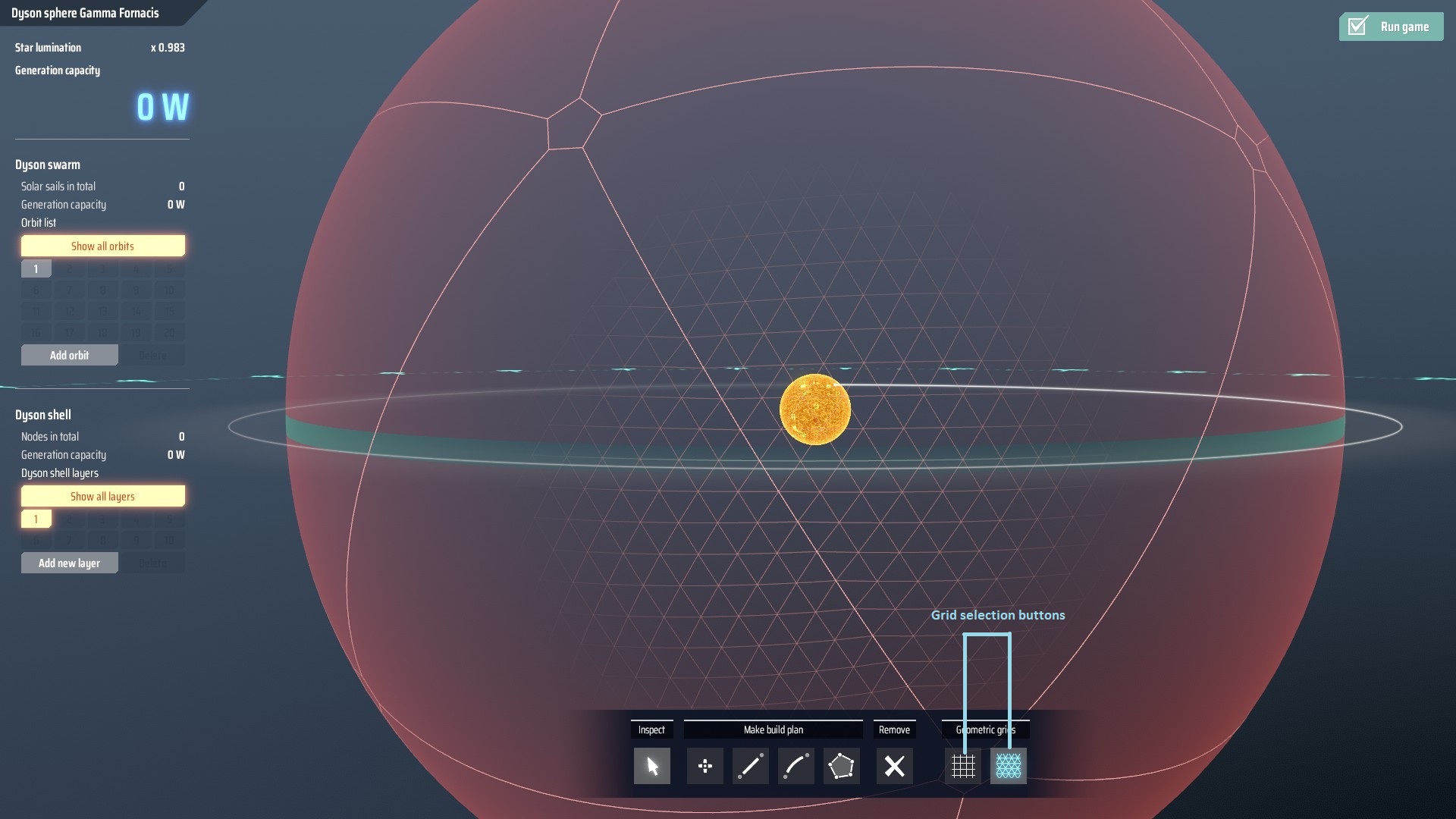Additionally we can change between two different grids with these buttons.
It should be noted that GRID SELECTION HAS NO IMPACT ON DESIGN. Those are only guiding lines to help you design a Dyson sphere, and you can change the grid at your leisure and any given point in time with no restriction.

Additionally – what may not be immediately obvious – you can get rid of the grid altogether by simply clicking on active grid again, and you will NOT be constrained by the layout itself, as shown here with no Dyson Sphere Stress System research:
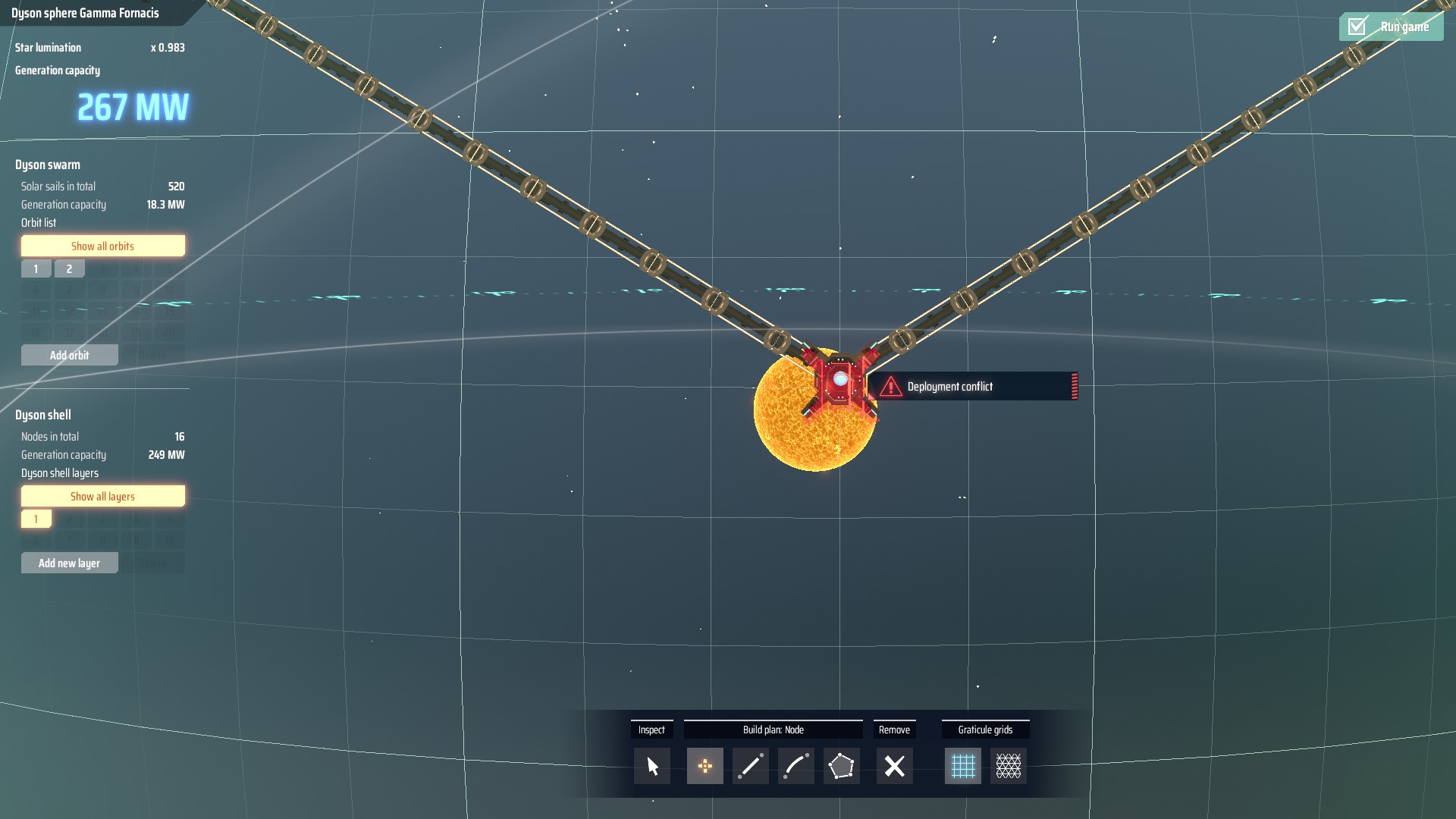
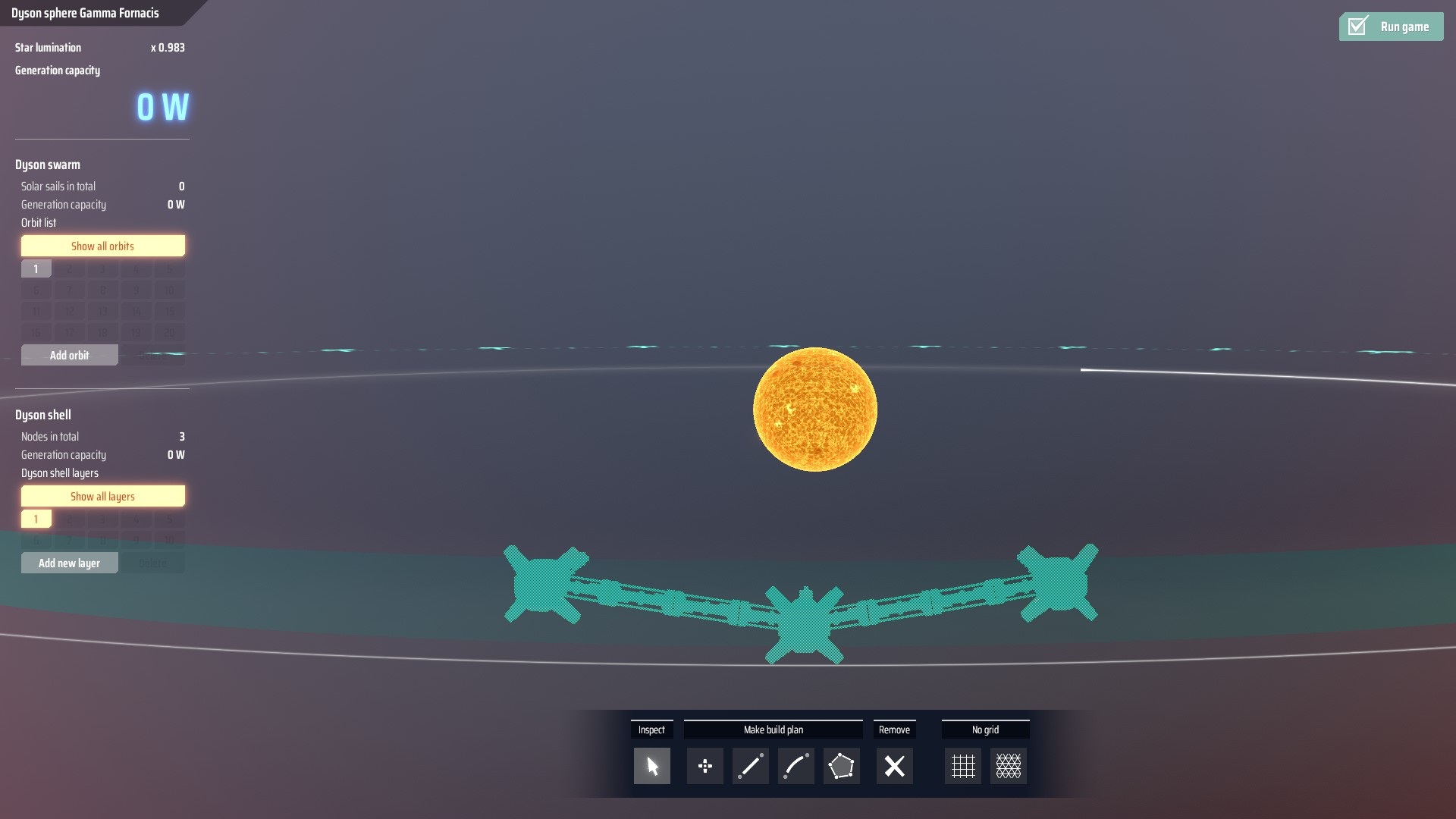Please be advised that there are still minimum connection angles and distances in this mode as well as with any grid.

At this point I can only encourage reader to play with those mechanics if they hadn’t done that already.

Every node and link has to be completed before it can support ‘shell’ areas. The cost of each node, and its’ capacity can be seen by clicking on the node itself. The cost is listed as ‘structure points’.

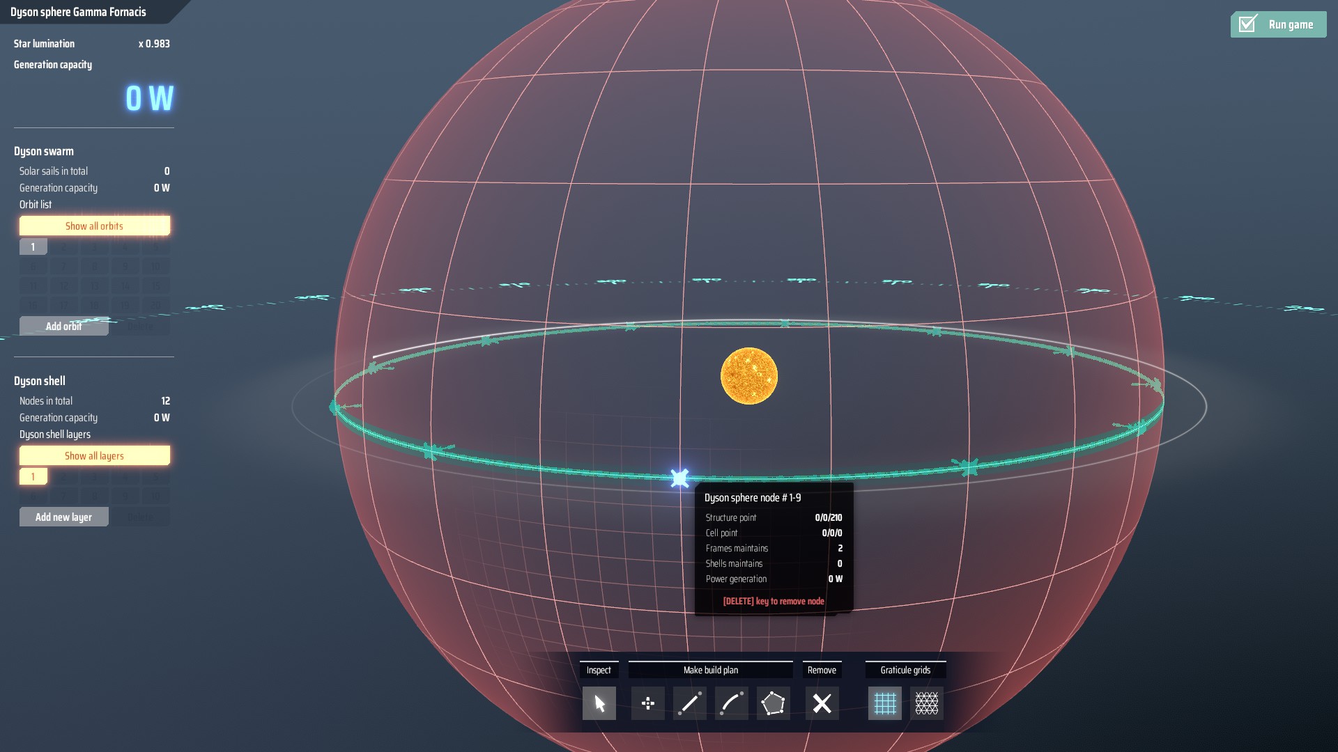
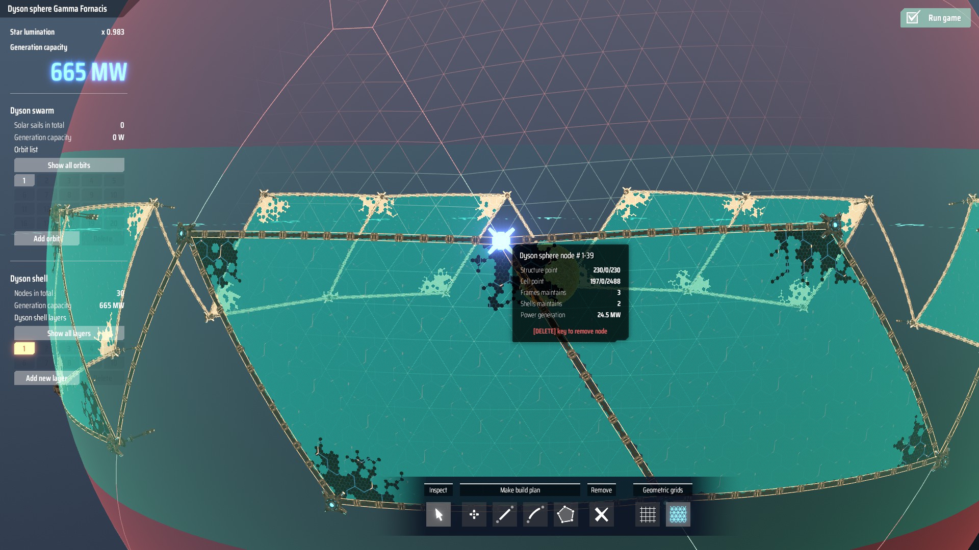
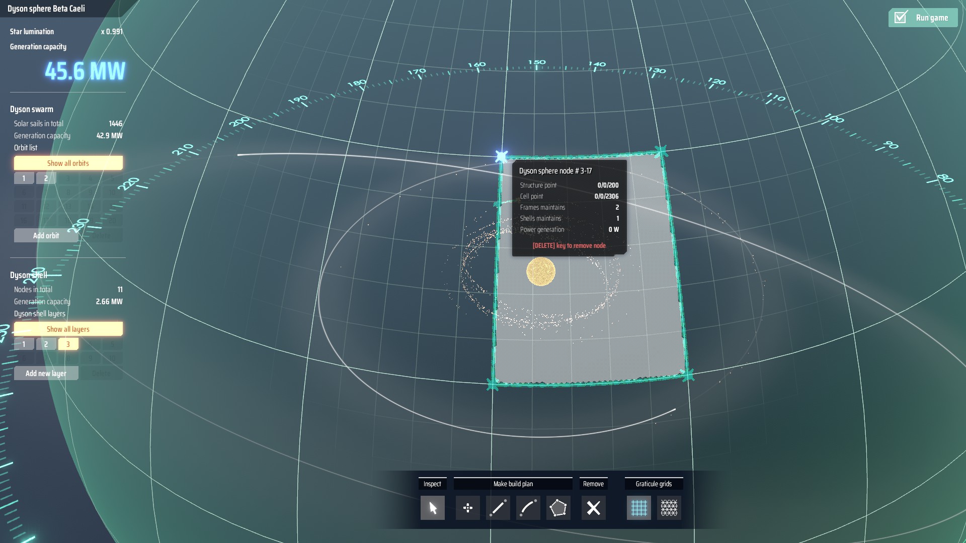
The numbers at structure points part of screnshot are from left to right:
– Structure points completed
– Rockets inbound (equivalent to structure points in construction)
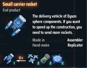
– Structure points total

Each structure point is equivalent to 1 small carrier rocket launched from a vertical launch silo.
Both elements can be used once Vertical Launch Silo is researched, and structure cannot be started without that research.

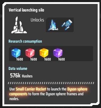
It also makes for easy calculation of a cost per structure point:

(exact cost after breaking down into raw materials is shown later in this guide).

For a Dyson Structure to be constructed, at least part of the sphere has to be designed.

THERE IS NO USABLE DESIGN AT THE START OF THE GAME.

This means that unless reader designs a sphere, no construction can be done even after supplying small rockets into launch sites.
Warning: Launch sites are extremely power hungry.

It should be noted that there is no known limit to how many carrier rockets can be sent at the time to a single node, with a note that no rockets will be sent if rockets in-flight and being launched will fill the demand for structure.
This basically means that you won’t waste rockets during construction, when you need 1 rocket, and have 5 silos ready to launch rockets.

Please note: you cannot create a shell without Dyson Sphere Stress System research of at least level 1.

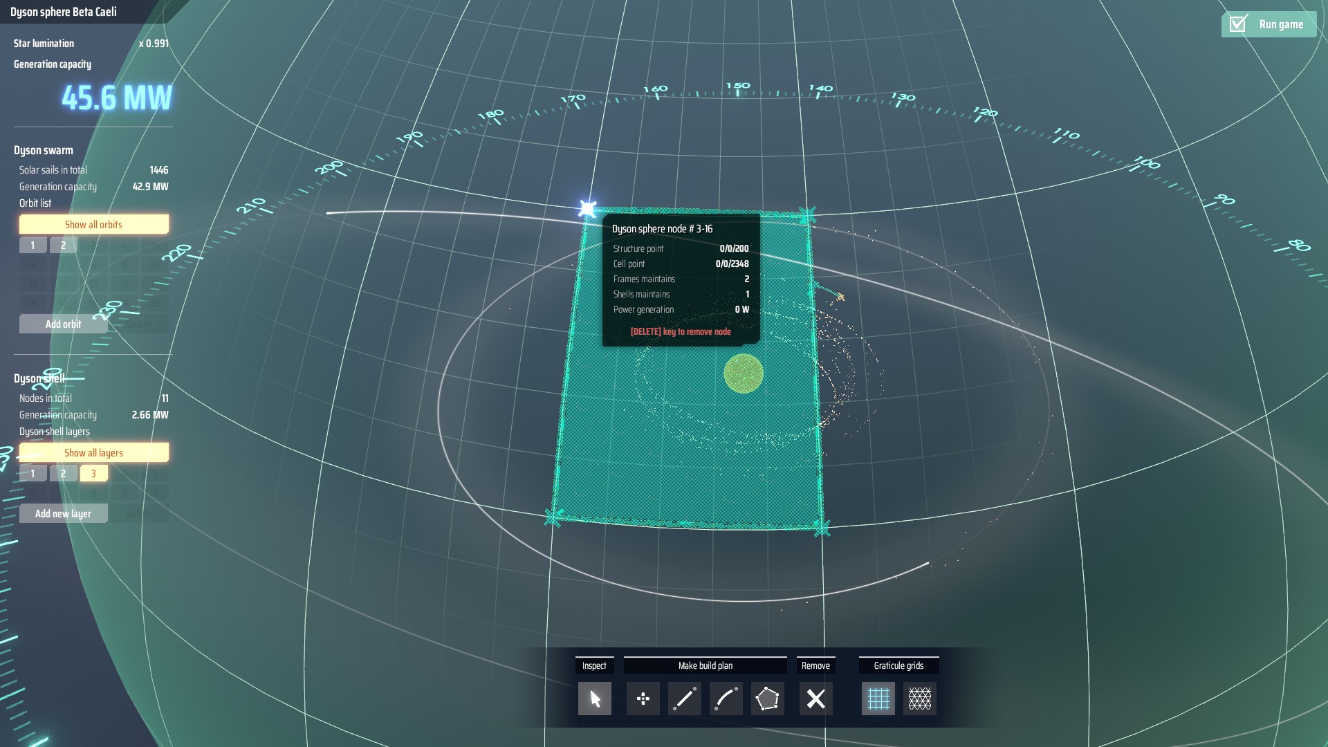
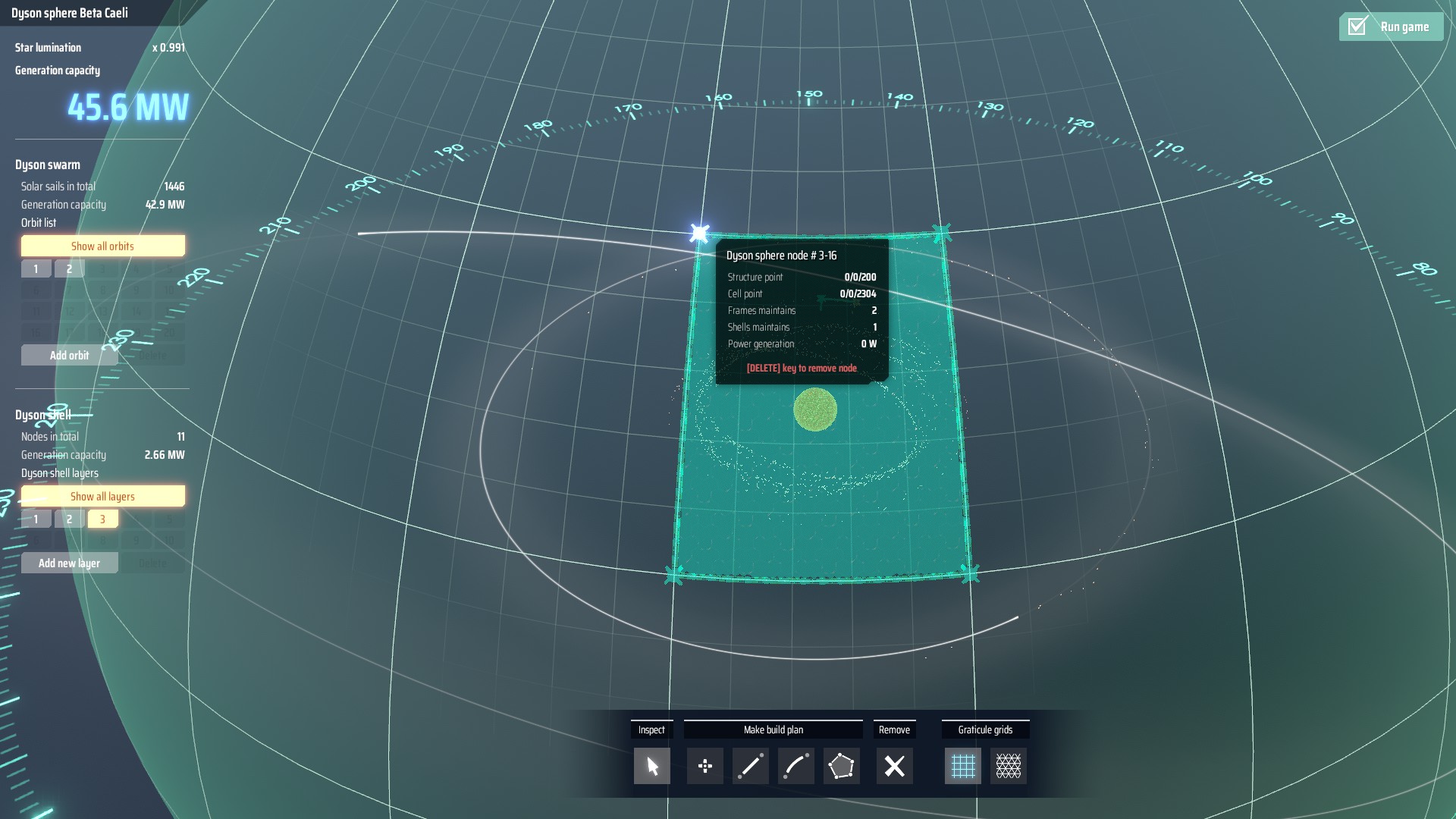
Every shell has predetermined capacity for ‘Cell Points’, as shown above. Once frame is designed a shell area can be defined within that area. Once frame part is completed node will request solar sails as cell points. Only built nodes can integrate cell points.

Shell can be designated before frame is complete, however shell integration process will only start after the node is complete [structure points are at 30 or above].

Cell points are acquired by automatic integration of Solar Sails from a Dyson Swarm. This process is automatic, but with limited speed at a ratio of 1 solar sail -> 1 cell point. Each node can control integration of at most 120 solar sails at the time, which leads to major delays in speed of integration. Exact time to integrate is not yet known, I will be doing some research in that topic, however I am unsure if reliable data will be produced any time soon. If anyone is interested in helping in that aspect please let me know.

It should be also noted that while exact orbit of Dyson swarm may have an impact in speed of integration, no data has been compiled about that yet.

Any Dyson swarm orbit can be used for the purposes of integration, and no manual activity is necessary. During and after integration no solar sails will be destroyed.

It should also be noted that Solar Sails LOSE EFFICIENCY once integrated into Dyson Shell, but at the same time GAIN INFINITE LIFESPAN.
In essence each Solar Sail reduces its’ generation from approx. 36 kW at luminosity 1.000 to approx. 15 kW at luminosity 1.000 [details in the power model], but no longer expire.
This in turn makes it so power wisely it may take few hours for integration benefits [lifetime increase] to pay off, depending on the time of integration in relation to total lifetime of that specific sail, and solar sail lifetime technology.

Standard Dyson swarm launch array can be used without any modification in shell integration.

Power Production model

Dyson Sphere Program uses custom power production model that does NOT conform to expected performance of real-life theoretical Dyson Sphere [DS]. Few key points to keep in mind when talking about in-game DS:

• There is no occlusion mechanics for power production in Dyson Sphere Program; This means that number of shells have no effect on power production at any point in construction. [that’s a big one] [It also has implications on power retrieval and solar power production].
• both structure points and cell points generate power scaled linearly to luminosity of a star over which DS is constructed, and luminosity can be used directly as multiplier to baseline values [at 1.000 luminosity].
• distance from the star’s surface has no impact on the power production of the sphere per structure/cell point
• every structure point and cell point has the same power production as any other structure point and cell point respectively [this means that e.g. a node with 1 structure point complete will have 1/30th production of a node with 30 structure points completed]. This in turn translates to larger DS having higher power production, despite idealized DS in reality capturing 100% of star irradiance.

Power production at luminosity 1.000

• Structure Point – 96 kW
• Cell Point – 15* kW

Notes:
Structure points were calculate directly by sending a single construction rocket in multiple systems. Dividing actual power by luminosity an estimate of 96 kW at luminosity 1.000 was made; Experimental verification was made thanks to azhur_2005, as shown above.

* – Cell points were derived from total power production – estimated structure point production, as per note above. As calculation was made recently, and estimated cell production is low [and rounding down is an apparent issue] – this value may not be as precise. Further experimentation will be performed.

Case Study [Predictive capability and accuracy]

For example of power estimation calculation we will use two spheres; One is my own, with documented construction progress on 3 stages; Second was provided by Zanthra (via Discord)

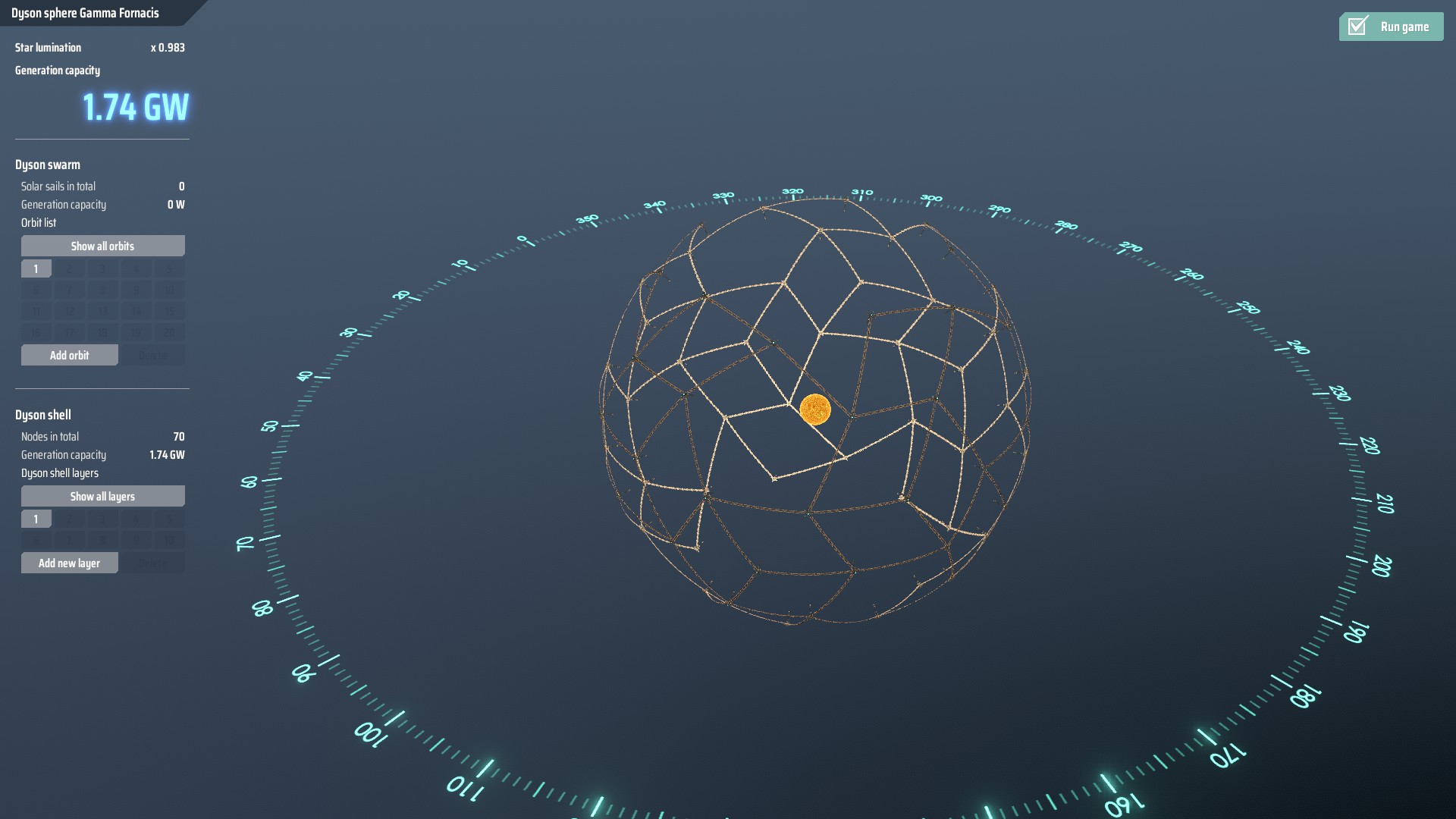
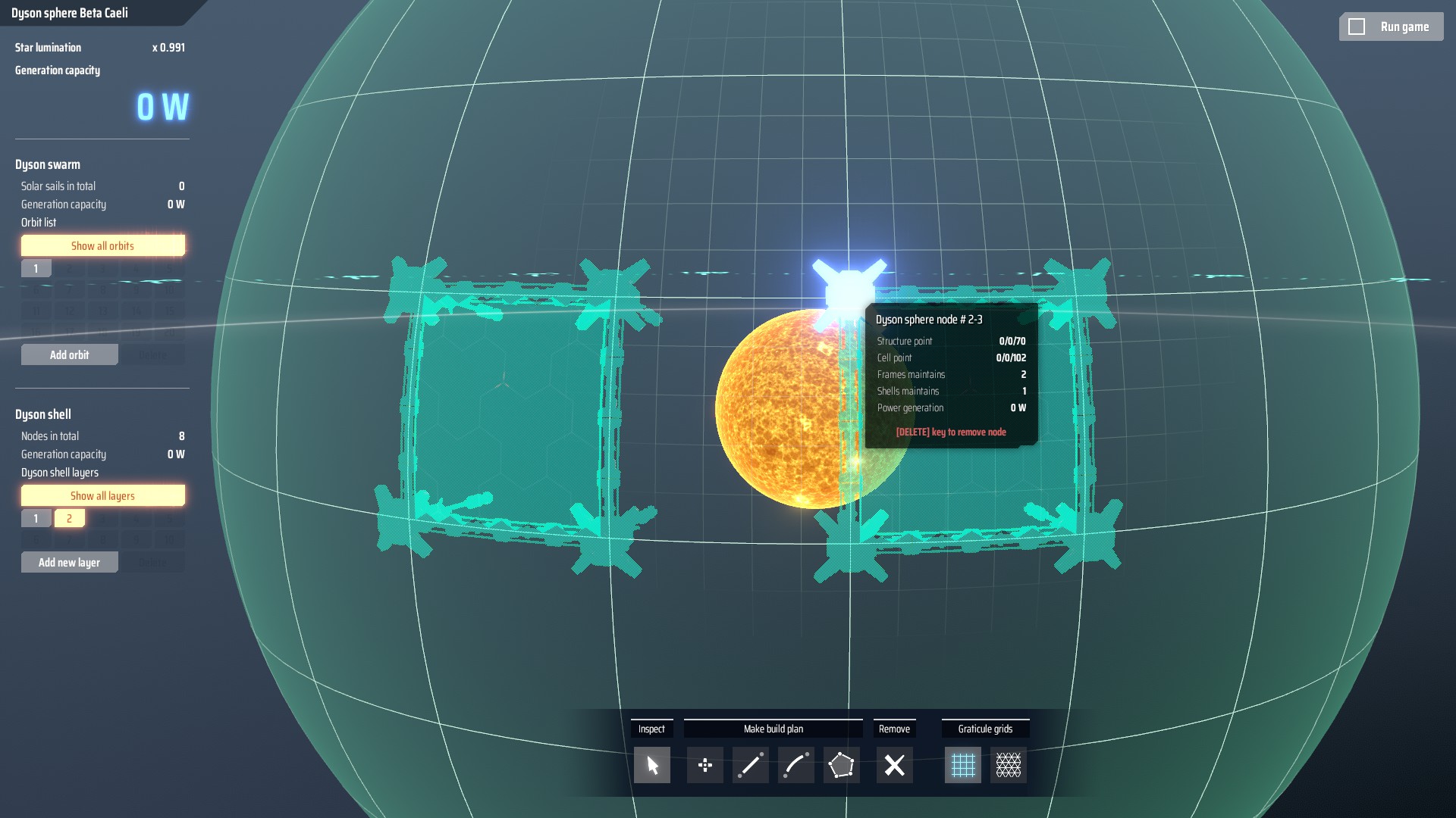Total structure points: 70
Total cell points: 102
Star luminosity: 0.991

Expected structure point energy production:
96 kW * 70 (number of structure points) * 0.991 luminosity modifier = 6 659.52 kW
rounding down 6,65 MW will be shown

Result of structure completion:
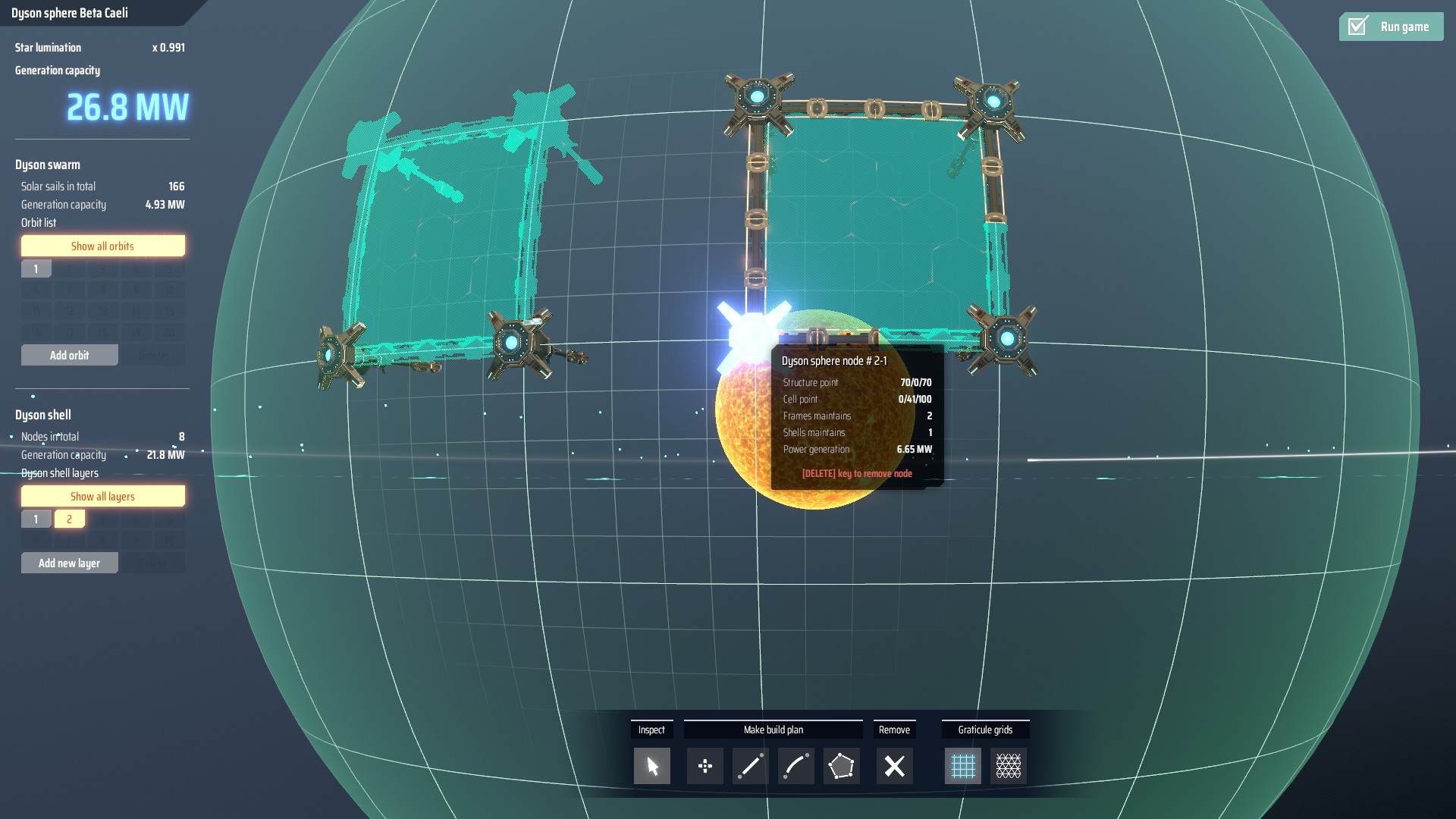Full match; Note though – the node is slightly different due to my mistake when creating a screenshot. Location on the sphere however has no impact on power production.

Expected cell point production:
15 kW (base production) * 102 (number of cell points) * 0.991 luminosity modifier = 1 516.23 kW

We are unable to see cell points alone, therefore we will add cell points’ expected production to structure points’ expected production:
1516,23 kW + 6659,52 kW = 817575 kW
Expected production after rounding: 8,17 MW

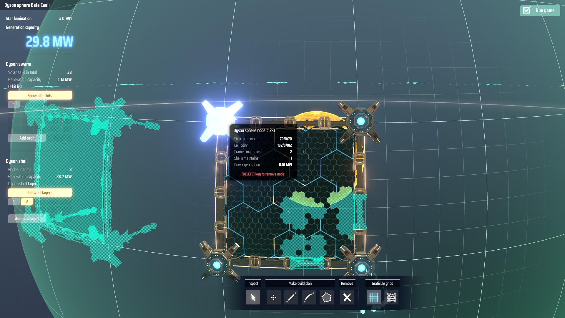Actual production shown – 8.16 MW

Deviation (expected production/actual production) = 1.001225490196078, or 0.13% of overestimation based on expected production;

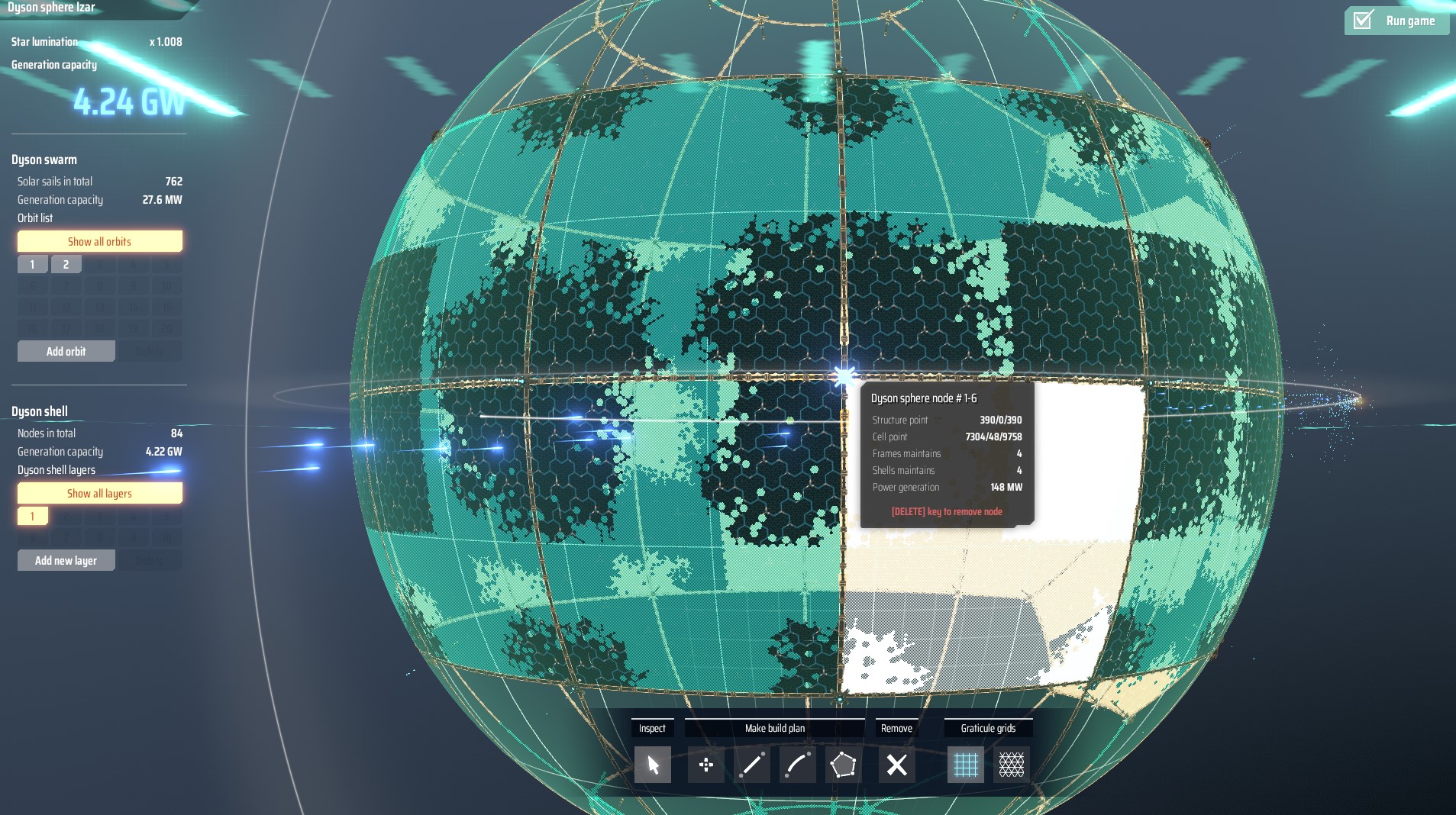Screenshot by: Zanthra

Total structure points completed: 390
Total cell points completed: 7304
Star luminosity: 1.008

Expected structure point energy production:
96 kW * 390 (number of structure points) * 1.008 luminosity modifier = 37 739.52 kW

Expected cell point production:
15 kW (base production) * 7304 (number of cell points) * 1.008 luminosity modifier = 110 436.48 kW

Expected node production in state shown on screenshot:
37 739.52 kW (structure points) + 110 436.48 (cell points) = 148 176 kW
148.176 MW, which is expected to be rounded to 148 MW which matches the shown value.

Cell Points count

Author: Danielosama

When selecting the Nodes that form a Shell, we can see the number of Cell Points each Node allocates. This number seems random at first, however, if we add the Cell Points of each Node that forms a Shell, the sum will always be consistent.

Here are some videos where we test and demonstrate it:

[1] Square Shell Testing:

[2] Triangle Shell Testing:

As you can see, no matter the number shown by each individual Node, when we add all Cell Points of the Nodes forming the Shell, it results in the same number.

You might have noticed that we tested both Geodesic and Graticule Links, that is because they slightly alter the number of Cell Points, as explained in the following section.

Links Type Effect

The following three screenshots are made with 2 types of links using the same area on the sphere. First and third screenshots are exactly the same for the purposes of design.

It should be noted that geodesic frame shape seems to have slightly higher number of cell points and each shell has fixed amount of cells, and only the node assignment is different. See more details above.

Sphere construction cost

It should be noted that every single cell point has to be filled by 1 solar sail.
For the purposes of this calculation only base recipes will be used. No rare materials will be taken into account during calculation.

Every cell point is a solar sail integrated into dyson sphere from standard dyson swarm.

1 Solar Sail can be divided into 0.5 graphere and 0.5 photon combiner; If we divide it further we will get raw materials of:

• 3.5 – stone
• 0.5 – iron ore
• 0.3 – copper ore
• 1.2 – oil
• 0.3 – water

This translates directly to cost of:

• 0.2(3) – stone
• 0.0(3) – iron ore
• 0.02 – copper ore
• 0.08 – oil
• 0.02 – water

for every 1 kW of cell point power at 1.000 luminosity star.
Please note that these amounts are NOT valid for dyson swarm power output calculation.

1 structure point is equivalent to 1 small carrier rocket launched from vertical launch silo; Each small carrier rocket costs [after calculation, and reduction to base materials]:

• 93 – iron ore
• 92 – silicon ore
• 39.5 – copper ore
• 80 – titanium ore
• 113 – stone
• 51.5 – water
• 159.8 – crude oil

This translates to:

• 0.96875 – iron ore
• 0.958(3) – silicon ore
• 0.411458(3) – copper ore
• 0.8(3) – titanium ore
• 1.17708(3) – stone
• 0.536458(3) – water
• 1.66458(3) – crude oil

for every 1 kW of structure point power at 1.000 luminosity star.

Note: If anyone spots any mistakes in these calculations please let me know.]
Note 2: In case someone is unaware of the notation : (3) at the end of decimal notation stands for infinitely many 3s following that. Basically 1/3rd would be represented as 0.(3), which is equivalent to 0.333333333… and so on. In case of iron ore per 1 kW of solar sail it represents equivalent of 1 iron ore per 30 kW, or 1 iron ore per 2 solar sails].

Every node on the sphere costs 30 structure points, regardless of sphere radius. Additionally – connection points cost 10 structure points per ‘link node’ [red bounding box in the screenshot below], added to the CLOSER NODE. [This is equivalent of adding 5 structure points per link node to EACHJ of connected nodes]. The amount of link nodes is dependent on radius of Dyson sphere, and is only contributor to the structure point price difference between large and small spheres. Only other price difference between two Dyson Spheres of the exactly same design is the amount of cell points needed to fill the cell point area.

Design Implications

Due to mechanics and costs there are 2 main design philosophies regarding DS construction.

This design will focus on maximization of structure points in any given design. This means that designer will want to reduce the length of every node, and connect every node to multiple other nodes around the main node to maximize amount of connection points. Keep in mind that amount of nodes and connection points between nodes reduce available amount of cell points in the shell.

It should be noted however, that this design philosophy is extremely cost inefficient due to amount of resources required to construct this type of DS.
Due to ability to construct multiple layers of DS over a single star this design is NOT recommended for non-‘infinite’ resource settings, as the limiting factor of this design is either resources available, or (when layered) construction area of planets used to receive the energy from the sphere.

This philosophy is focused on maximization of cell points and reduction of
This means that designer will attempt to reduce amount of nodes and links to minimum, while increasing the area of cell elements.

It should be noted that this design is power sparse. As in – in the same area power density could be increased by use of different design; This design, when layered may still cap efficiency based on amount of construction area of planets within system.

Due to game’s Dyson Sphere NOT taking occlusion into consideration [at all], the maximum amount of energy could be obtained by creation of default sphere at radius 10 000 and 9 additional shells fully constructed with power density design philosophy. It should be noted that 2 shells have minimum radius difference of 1000. This means that two closest shells to 10 000 radius shell would be 9 000 radius and 11 000 radius. Maximum power possible would be obtained by layering starting with the largest possible radius, and other shells with radii reduced by 1000 per shell layer.

As solar sails only need 30 points of structure on the node to start integration AND there is no apparent relation between the amount of solar sails you can integrate and number of finished structure points – it is possible to pre-plan entire dyson sphere by using nodes alone, then go as far as remove all rocket launch sites, design node links, and fill the shells in design. All integration should start and be completed without any introduction of structure points. It should be noted however, that this leads to reduction to overall power production, due to loss of structure point energy production.

Thank you Alavaria for noticing that.

Optimized Cost Efficiency Design – True Football design by Oleg

This design is created with cost efficiency in mind, by minimization of node quantity and minimization of node links.

Design was created by Oleg, and is probably the optimal design for a Dyson sphere when it comes to minization of link length. Unfortunately it does not follow precisely any grid, and as such may have some elongated nodes.

Reference data: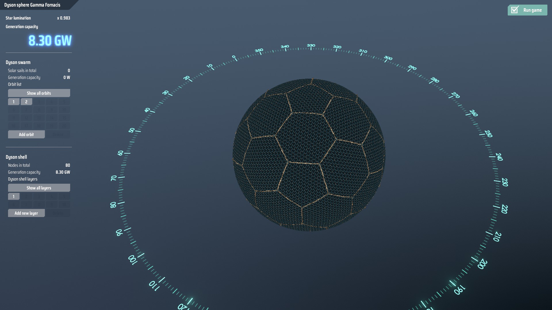
approx. 8.44 GW
16 800 structure points
(approx. 27.1 cell points/structure point)

While the following design steps are designed around full dyson sphere stress system research, this design can be constructed step-by-step starting at DSSS level 1;

First things first – this design is heavily symmetrical, and just like previous football like design uses the Geometric Grid Layout.

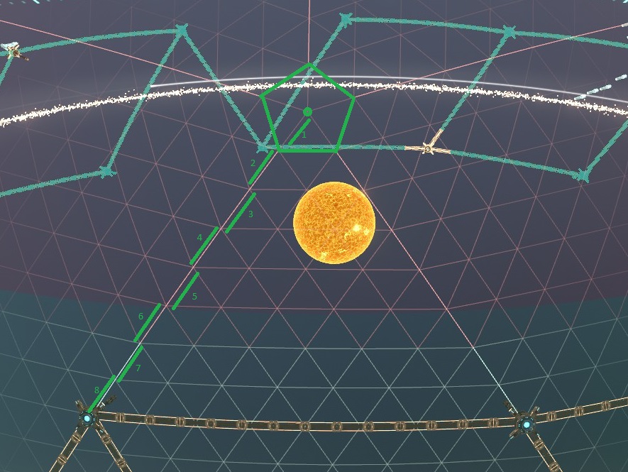
Geometric Grid layout has few focal points, and this design also uses length of 8 to go through the nodes, however rather than edges, we will use 8 heights of triangles in the design, and as we will be following regular sets of 8 heights – we will calculate distances using 2 connected triangles creating a rhombus. Let us calculate distance of a pentagon node from the focus point, as shown below.

It should be noted that the center node is here only to show where the focus point is, and to show the distances and calculation of distances.

Once all focus points are covered we can extend that distance by another 4 ‘units’, and connect nearby pentagonal sections:

Once all connections are made entire sphere is divided into both pentagonal [near the focus points], and hexagonal sections. Please note – hexagonal sections will NOT be uniform.

At this point we can fill all spaces in those sections with shells, as all of them are small enough to be filled, and large enough to require no further connections.

While changing the grid type, it may seem as if it is following both grids, however it is not the case.
There is small discrepancy between the grids as shown here:

Improved Cost Efficiency Design [Deprecated]

Deprecated by optimized cost efficiency design.

Original improvement over previous cost-efficiency design [which is linked below in this guide], was provided by Oleg (Click here for original improvement screenshot) I have also tried to improve on that by reducing the total length of links between nodes; I did it by movement of few of the nodes closer to the equator of the sphere, to approximate the cap segments closer to squares.

Reference data:
19 300 structure points
Total power production at 1.000 luminosity:
~8.67 GW
(approx. 23.57 cells per structure point)

After creation of first layer at Dyson sphere stress system level 2, at 4th level we extend every 3rd node [so that we get 4 ‘pillars’ added], and then add an intermediate node at the middle between two original nodes, and 6 spots up.

This is the middle point between the nodes: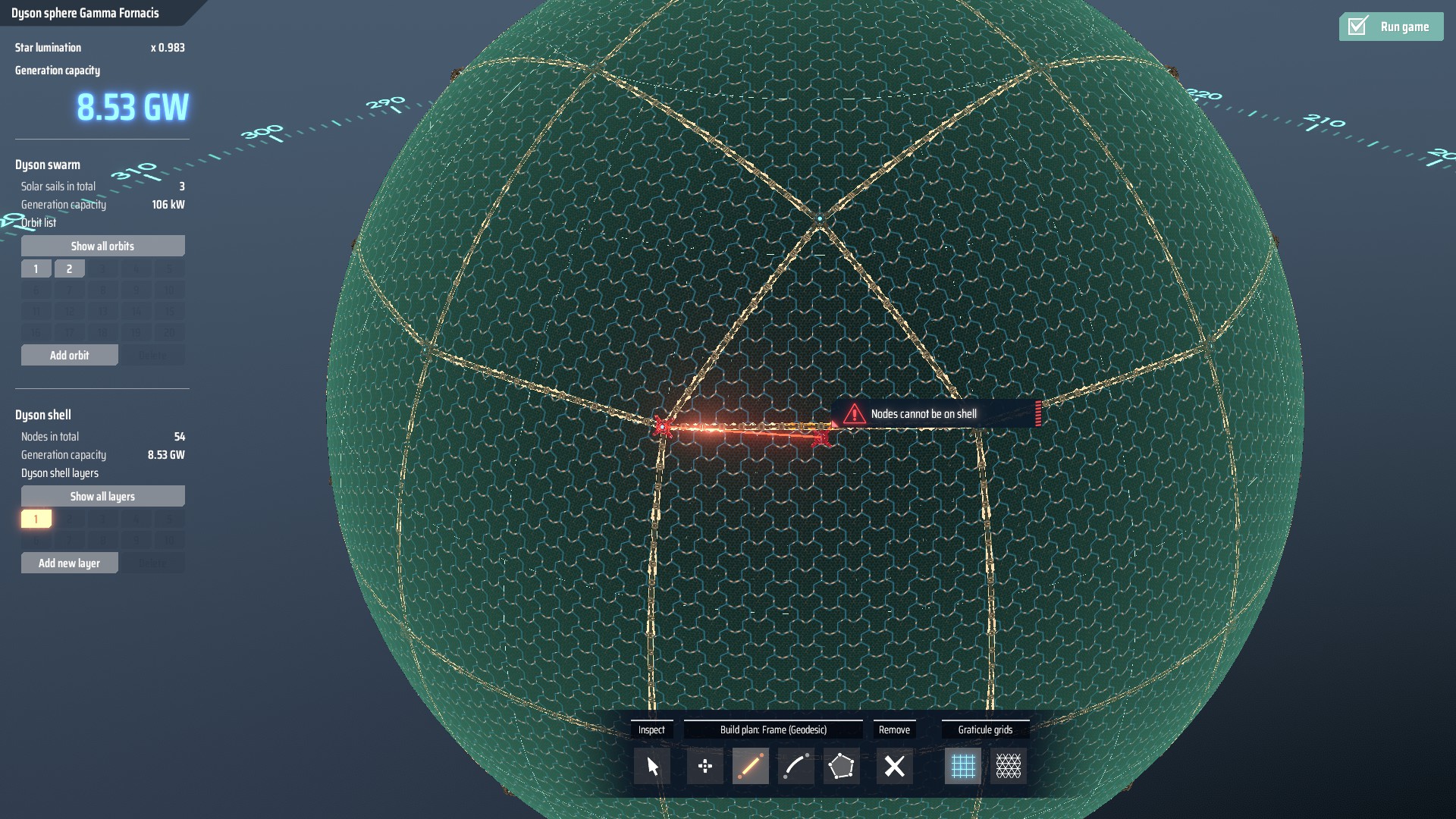

And length of 6 node positions:

This position allows to save 40 structure points per triangular node [total of 320 nodes across entire structure] in relation to original design at 10 000 radius Dyson sphere.

Cost Efficiency Focused Design [Deprecated]

The following design is created around the idea of cost efficiency, in form of reduction of connection nodes to minimum, with minimal possible link lengths.

Deprecated in favor of design shown above, though it should be noted that improvement is relatively low.

Reference data: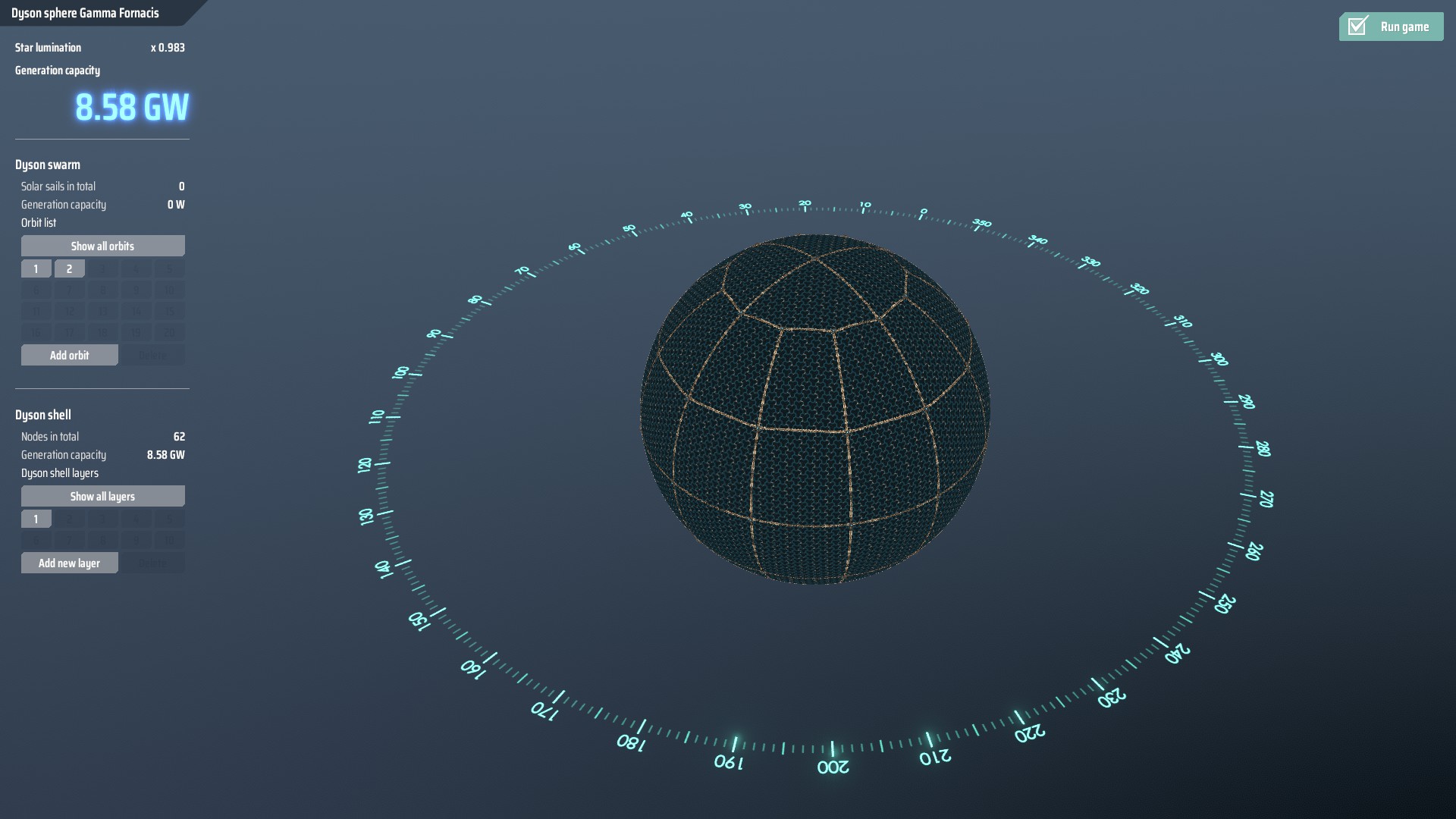

19860 structure points
Estimated production at 1.000 luminosity:
~8.71 GW
(approx. 22.83 cells per structure point)

This design has a high efficiency, but requires level 6 Dyson Sphere Stress System to be completed, due to cap having a center-node on the poles.

Alternate version, that skips the requirement of level 6 DSSS would have cap like this one: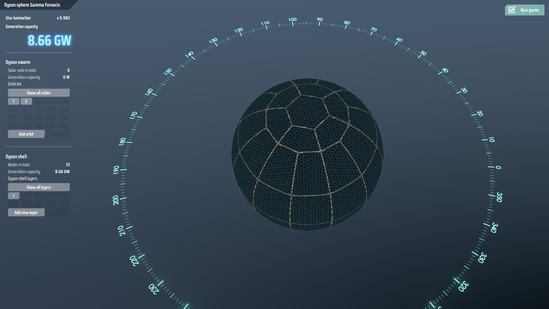

20660 structure points
Estimated production at 1.000 luminosity:
~8.81 GW
(approx. 22.02 cells per structure point)

It should be noted that the ‘core’ is made by creating a ring with 12 nodes around the equator, and on Dyson Sphere Stress System levels 2 and 4, the sides are extended as far as possible, and square areas are created by connection of the newly extended nodes.
It is also possible to add minor optimizations by reducing amount of ‘ring’ nodes, and it’s been tested with 4 at minimum, that forms a square cap pattern:

(note: NOT a reference radius in this case)

Power Density Design

The following design is created around the idea of power density, in form of maximization of structure point by means of number of nodes and amount of connection between the nodes..

While this design is a strong candidate for one of the most power dense designs, it should be noted that I have no intention in claiming that is the most cost efficient design possible. This design was created using geometric grid, and is quite possibly the densest design available using this specific grid, however it should be possible to create even denser design using no grid option, and there may be means of increasing this density beyond what I have taken into consideration.

Reference data: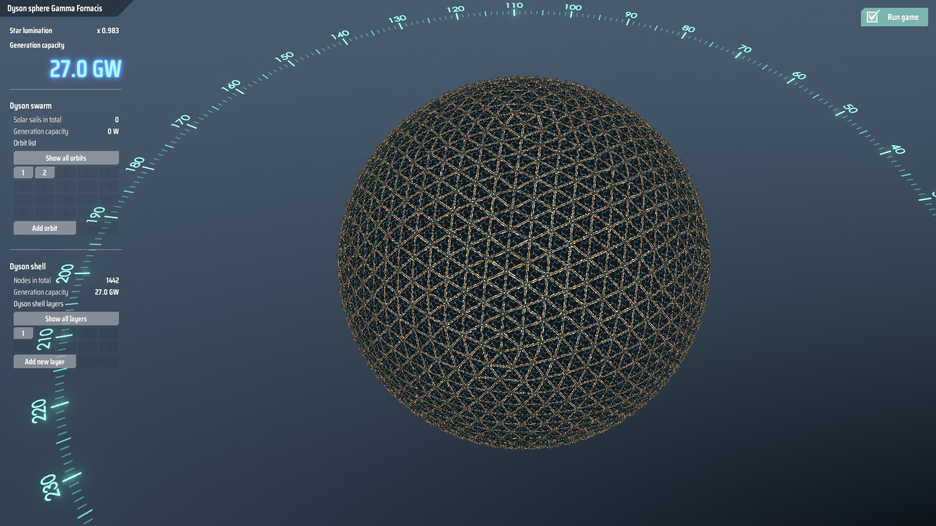

216 060 structure points
Estimated production at 1.000 luminosity:
~27.46 GW
(approx. 2.07 cells per structure point)

While the power output of this sphere is more than thrice as high as second most powerful design [energy wisely] in this guide, it should be noted that this design has the cost of construction of over 10 times than that design.

This leads to extreme construction costs and construction times, with a bit more than 720 launch-hours to complete. This translates to around 72 launchers active for 10 hours straight to complete this design.

On the flip side this design has extremely high efficiency in solar sail integration due to number of nodes that can concurrently accept solar sails, as well as low total number of solar sails needed per node, pushing this design into structure limited completion time.

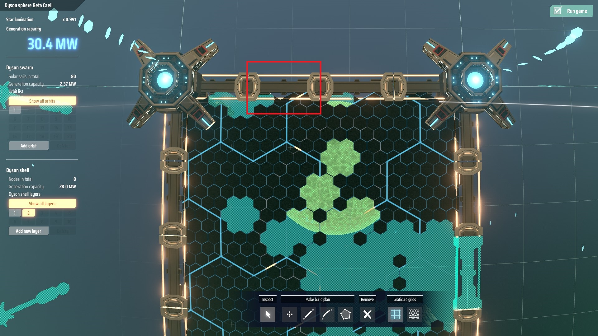
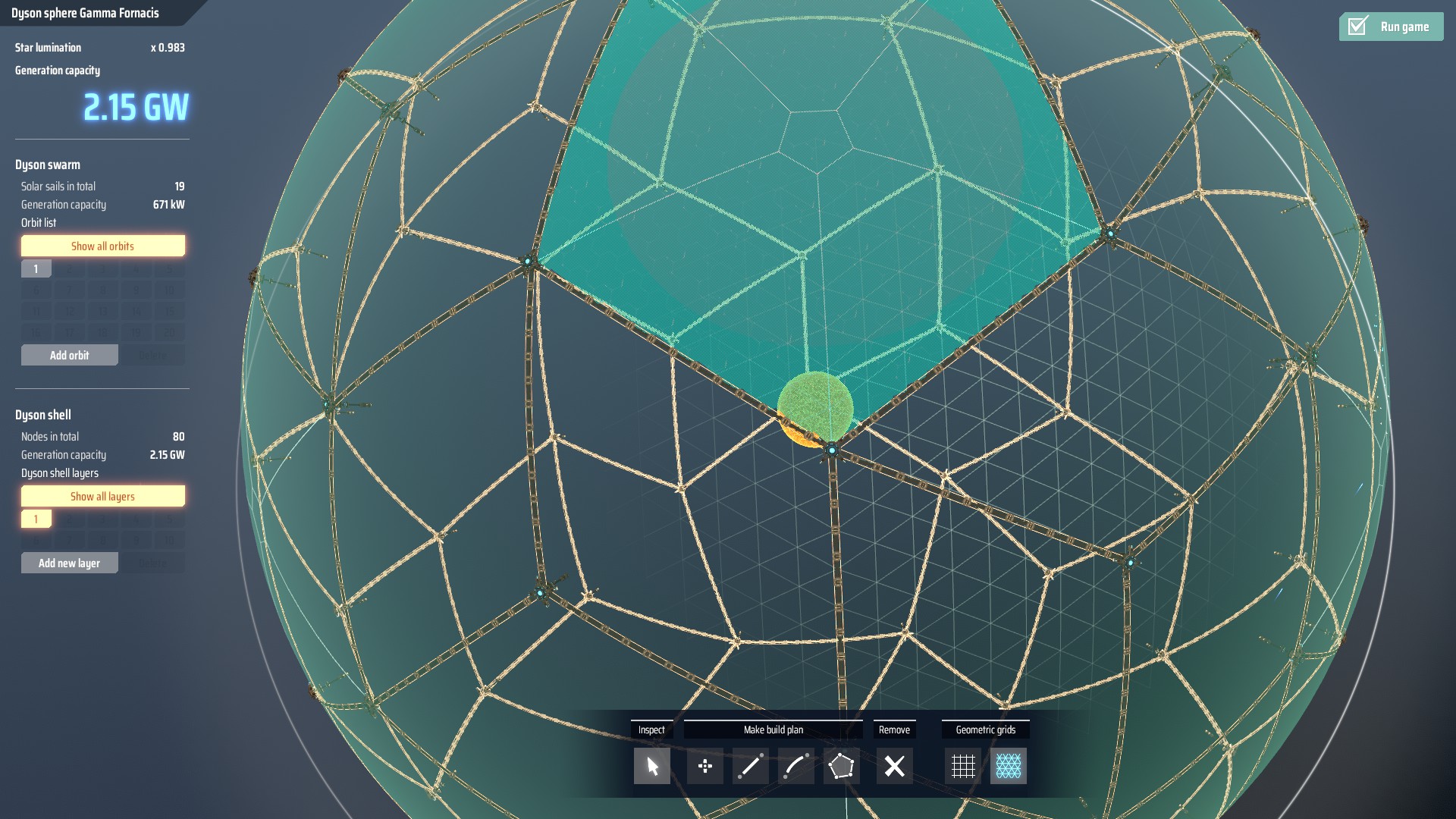
‘Football’ Design Dyson Sphere

This section will describe construction of a ‘football’ design Dyson Sphere in detail.

This is a reference screenshot of complete football design sphere: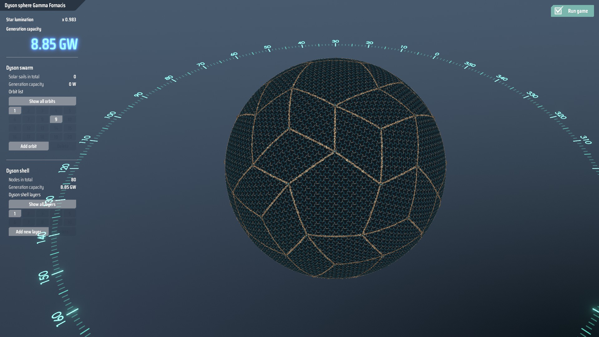

Taking this in mind default shell these are information of this design for comparison purposes:
approx. 9 GW
22 800 structure points
(approx. 19.9 cell points/structure point)

Design features:
– This is regular design, without pronounced equator.
– Relatively high cost efficiency, with 80 nodes necessary to cover the sphere
– MAJOR WEAKNESS – Design cannot be started without Dyson sphere stress system level 1 or higher.
– Strength – Design does not require Dyson Sphere Stress System to complete. Research is redundant with this sphere.

Dyson Sphere Stress System will be abbreviated as D3S.
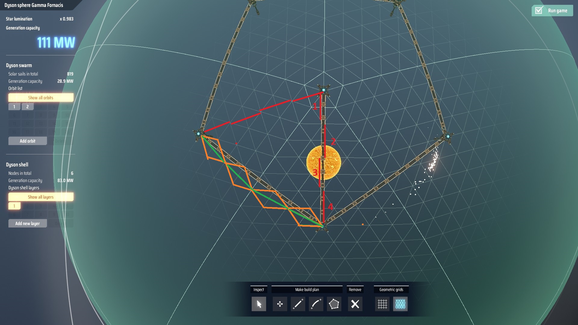
Entire design will be done using GEOMETRIC grid layout.

D3S level 1;
We start with set of regular structure:

To do that we take care of the following steps:

• Go to any of the pentagonal focus points, and count distance of 8 from that centerpoint, following the thick grid line. (see detail screenshot)
• Place a node at that distance;
• Follow one of the ‘side’ grid lines, 8 tiles to the side; It should be in-line with another thick line. Connect this node to original node]
• Follow the thick line for another 8 tiles [ALL lines in the design are 8 tiles long leading to extremely regular shape] and place another node there.
• From the bottom line go to the same side as in point above to add parallel line to one you set up before.
• Connect two rhombi in a line, and connect them with an “N” method as shown in the general design.

D3S Level 2:
Unfortunatelly D3S level 2 doesn’t give us enough space to add another node, so we have to skip it.

D3S level 3:

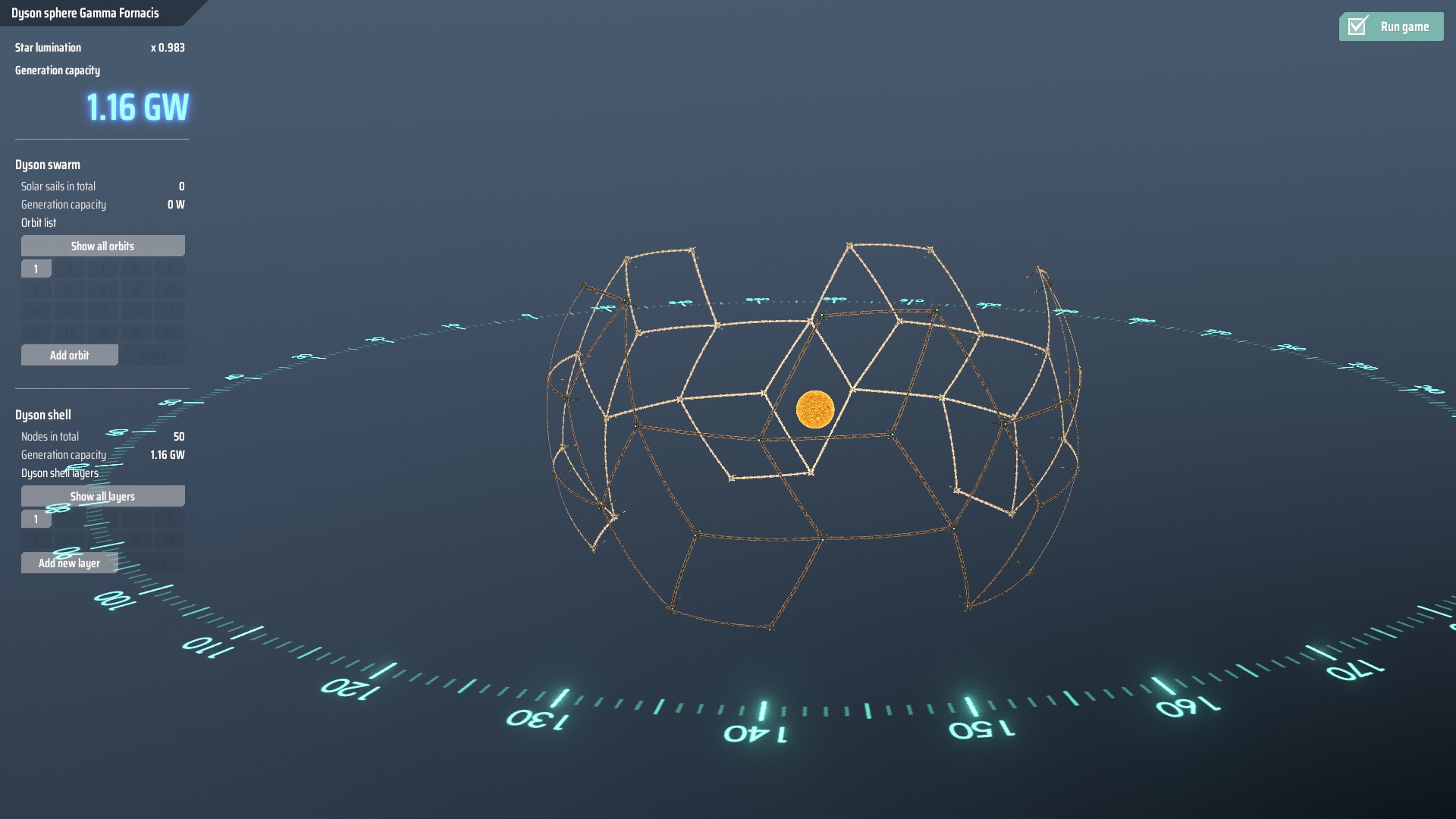
Here we can complete the hexagonal design we started previously; We can easily follow the geometric lines [with 8 line lengths each time] to complete the hexagons. Adding more connections from center of hexagon to the bordering nodes will reduce cost efficiency, but increase the power density; so keep that in mind.

D3S level 4:

At this stage almost entire structure is complete; Some of the heptagons are complete, and only thing left to complete are the pole heptagons. Luckily we can simply continue building both regular rombi and hexagons to complete this stage.

D3S level 5:

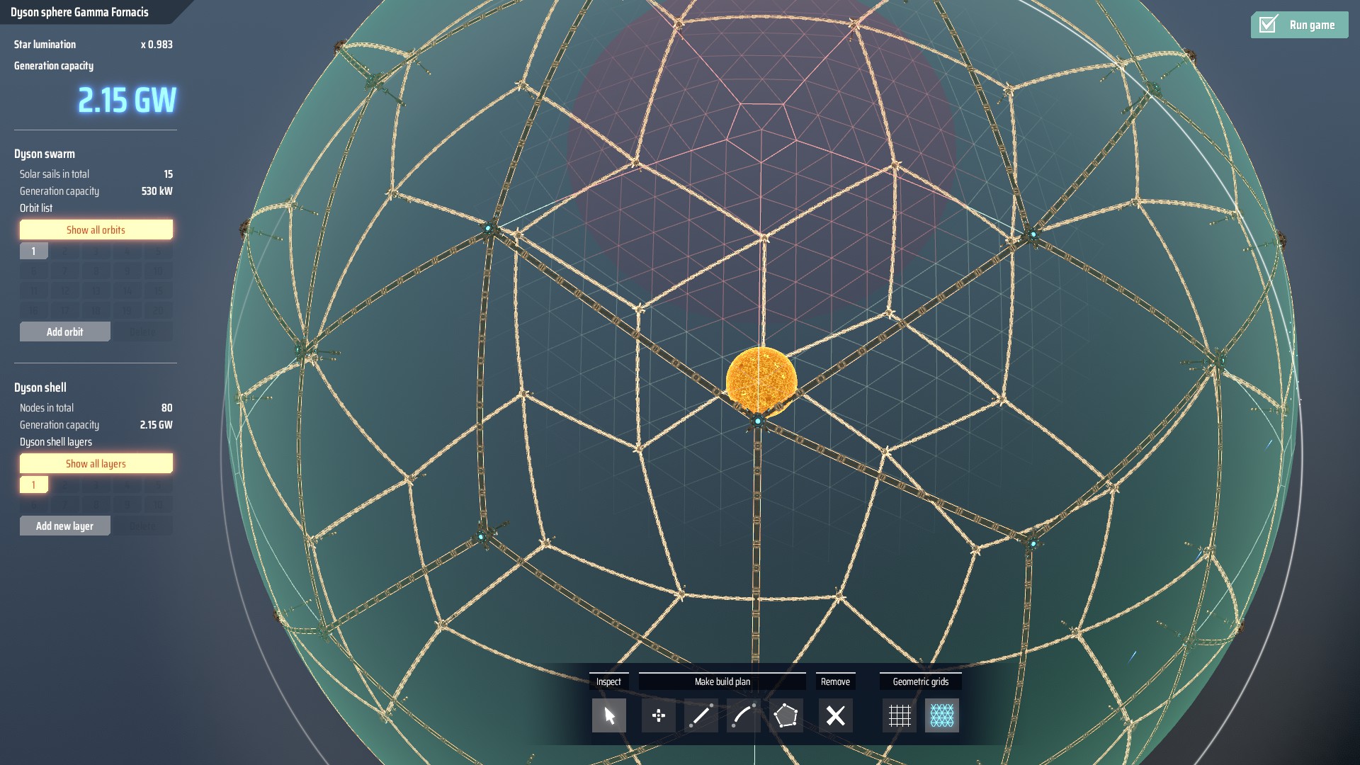
Finally we can complete the design on this level; Despite having no ability to add nodes in the pole section of the design, this are can be filled with shell without technological issues.

At this point football design is fully complete.

Please keep in mind that guide focuses on structural part of the sphere. At any point in design once area is ‘closed’ [starting from D3S level 2] that closed area can be filled with a shell.
Guide doesn’t show filled version for the clarity of structure design.

Energy Retrieval from Dyson System – Basics

It should be fairly self-evident that the purpose of the Dyson sphere and a Dyson swarm is quite simple: Generation of Energy. While this purpose is quite clear, we have to keep in mind that Dyson sphere itself has no accumulators, and has no ability to store or use energy as-is.

To retrieve energy from any sphere or a swarm a Ray Receiver technology is required.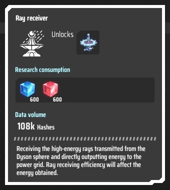

The ray receiver [from now on simply ‘receiver’] is the ONLY method in which we can take energy from the Dyson Sphere/Swarm and turn it into useful grid energy; either directly or indirectly.

It should be noted that usually the receiver requires direct line of sight [LOS] to any part of the Dyson swarm/Dyson sphere to utilize energy from the Dyson system.

I will start by listing the modes with their characteristics.
Please note that both mode pictures will be shown using exactly the same receiver, at full potential power modifier from the continuous operation.

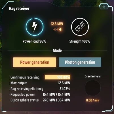
This is the default mode; It is available as soon as receiver tech is unlocked.

Strengths of this mode:

• No processing is needed, and energy can be used from get-go.
• No resource maintenance of this process.
• No research required to unlock this mode.
• Higher energy conversion efficiency from Dyson system into grid energy network. [It means that it has lower total loss of energy between when the energy is in sphere, and when it is output into the grid].

Weaknesses of this mode:

• Main weakness is it’s transfer density. While it can provide reasonable amount of energy early on, the photon mode can output a bit below 5 times the efficiency of this mode (exactly 5 times in photon generation; loss comes from processing of photons; more on that below).
• Due to lower transfer density – benefits of graviton lens is reduced.
• Outputs only as much energy into the grid as is needed, therefore it depends on accumulators for energy storage.

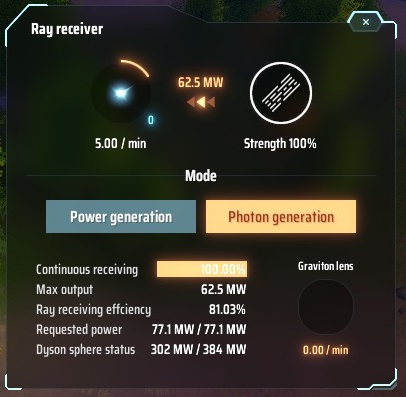
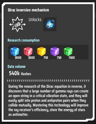
This is researchable mode. Instead of generating energy to be used in the grid, it generates photons that after processing can be used in late-game Artificial Star power facility. It should be noted that the main energy loss comes from division of critical photons into antimatter-matter duo, rated at over 120 MW. Additional cost comes from transfer of items via sorters and assemblers making components to the antimatter ‘fuel’ cell. Each critical photon ‘costs’ 750 MW from Dyson System.

NOTE: This node DOES NOT interact with grid in any way shape or form directly. It takes energy from Dyson sphere directly and outputs photons as a product.

Strengths of this mode:

• High energy density; This mode allows to obtain 5 times the amount of energy from Dyson system, and create a photon from it.
• Very high graviton lens efficiency. Due to high energy density – graviton lenses are extremely cost efficient in this mode, in comparison to normal mode.
• Due to energy being used to generate critical photons – this mode can be used as a power storage module from the dyson sphere perspective, as it’s full capability will be utilized at all times, and no accumulators are needed.

Weaknesses of this mode:

• Cannot be used as a self-starter design. Entire energy recovery process in this mode has to be provided with initial energy to reprocess energy into usable grid power. While a single planet and a single sphere can supply multiple production planets, in the event of critical power failure when this receiver is THE ONLY means of getting energy – no energy will be retrieved from the Dyson Sphere.
• Requires additional research to use.
• Conversion process of critical photons into grid energy requires additional resources: titanium alloy and annihilation constraint sphere, which are both using non-renewable resources in creation.
• Conversion process of critical photons into grid energy nets a NET LOSS of energy between energy ‘captured’ in form of critical photons and released using Artificial Star. This leads to effective reduction in efficiency over direct energy mode, assuming both systems work constantly in the same environmental conditions.

The technology required to use this mode is

Here I would like to add short note regarding graviton lenses. It should be noted that graviton lenses can be researched completely independently, however they won’t be usable in receivers until the planetary ionosphere research is complete.

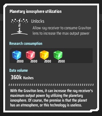
When inserted Graviton Lenses start using planetary ionosphere to increase total output of the receiver they are inserted in by 100% for the duration of 4 minutes for every lens.

It is a common question to ask what exactly specific parts of the receiver menu mean. I took a libery of adding a note to one part of the menu, to let me explain it in, hopefully, more accessible manner.

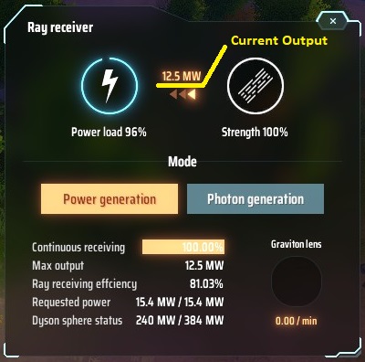
Current output is how much energy is inserted into the power grid or into generation of critical photons.

Continuous receiving is a strength of a modifier that benefits from the duration of receiving by the receiver. It simply means that the receiver will transfer less energy [starting at 5 MW] at the beginning of the day, or more specifically – when it starts ‘seeing’ the Dyson System, than it does in few minutes of continuous receiving. In standard mode, without lens it caps at 12.5 MW, as shown above.

Max output is the amount of energy that the receiver can push into the grid OR into a critical photon [depending on the mode]. Note – this amount does NOT change based on energy transfer loss technology level.

Ray receiving efficiency is information how much of the power sent by the Dyson System is accepted by the receiver. If it is at 40% it means that for every 100 MW that Dyson System sends, receiver can output 40 MW.

Requested power has two numbers, in the format: [received energy from Dyson System] / [total energy needed from Dyson system]. It should be noted that this value will be red if the Dyson System cannot output enough energy to fulfill demand from the receivers. Requested power tells status of this specific receiver. Total energy needed from Dyson System will be higher than maximum output power of the receiver. It is amount of energy that Dyson System needs to send, in order for the receiver to output its’ current maximum output.

And finally – Dyson Sphere Status, shown in format: ]total energy requested by the receivers] / [current Dyson Sphere output]. This, just like in above case, will be red if the sphere cannot output enough energy to fulfill entire demand by ALL receivers with line of sight [‘active receivers’] to the Dyson system.

The key issue here is the following: When energy in the Dyson sphere is not sufficient to supply all receivers, the energy given will be divided between receivers proportionally to the amount of energy they need. In simpler terms:
If we have 3 receivers with demands of 5, 7.5 and 10 MW, and Dyson System has transfer efficiency of 50% the Dyson system needs: 5*2 + 7.5*2 + 10*2 = 45 MW. [Multiplication by 2 because it’s equivalent to division by half, in this case – division by the efficiency of transfer. This way we can calculate by ourselves how much energy we need to send from Dyson System].

If we have only 15 MW in the Dyson Sphere, each receiver will get only 15/45 = 1/3 of what it needs. Therefore the receivers will get 1.66, 2.5 and 3.33 MW respectively.
The more energy receiver needs, the more it will receive proportionally.

Energy Retrieval from Dyson System – Implications, including non-obvious ones.

During energy retrieval part of the guide I often used term ‘Dyson System’. Primarily due to the fact that, unlike what some may think, receivers do not need to be in the sunlight. While that is area necessary for use by solar power, receivers do not take energy from the sun. They can obtain energy from any part of the Dyson system. This in fact means that one can create specific orbit for solar sails, for the purposes of extending the angle from which energy can be received from the Dyson System. In few cases, where such orbit goes beyond the orbit of the planet receiver is placed on – this can allow, by itself, retrieval of energy from anywhere on the planet with simple use of solar sails as a set of relay satellites. As long as receiver is in range of single solar sail or small part of the sphere – entire power system for the sphere is accessible.

As solar sails and dyson sphere have the same possible orbits, it may be of use to create a relay nodes without any links between them. Each node has the same cost, regardless of distane from the star – 30 structure points, and just like solar sails they can be used as relay nodes. This increases setup cost of relay system, but it pays for itself in the long run.

It has been mentioned in the guide before, but I deem it worth repeating. There is no occlusion system for purposes of power production in DSP. There IS an occlusion system for purpose of graphical shadow representation. It also means that in the event that direct line of sight is obscured by a gas giant [if the receiver is placed on a natural satellite of the gas giant, such as on starter planet], the gas giant will NOT impact energy retrieval of the receiver.

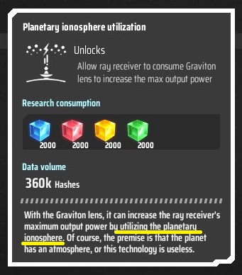
Full description of the technology makes a claim that the graviton lens allows the receiver to use IONOSPHERE of the planet as a means of receiving energy. Why does it matter? To put it simply – on planets with atmosphere, as long as receiver is using graviton lenses, the receivers can receive energy from anywhere that is within line of sight of ionosphere of the planet. In simpler terms – at this point in time for game purposes – from ANYWHERE on the planet. That includes the dark side of the tidal locked planets with no line of sight to any part of Dyson System.

Solar Power VS Dyson System comparison

Quite common point of contention is the solar power, or to be more precise – planet based photovoltaic pannels VS Dyson system comparison when it comes to power generation.

Let me start with a short preface – Neither system is strictly superior to the other, both systems have their own uses, and both have their own raison d’etre [reason of existence, just in case].

Before I start with full description, let me start with cost of planetary solar panel, and efficiency of one [at 100% solar efficiency planet, as standardized version].

Each solar pannel costs, after reduction to its base components:
– 4 iron ore
– 16 silicon ore
– 8 copper ore

and generates 360 kW of rated power at a planet with 100% solar cell efficiency.

This translated to cost per kW:
– 0.0(4) silicon ore
– 0.0(1) iron ore
– 0.0(2) copper ore

If we use stone ore instead [extremely NOT recommended, for comparison purposes only]
we get 0.(4) stone per kW.
In essence we have difference in silicon/stone cost and iron cost between this and solar sail. What is curious is that it is a difference that makes solar panels more cost efficient option, and that’s… partially true. As they say – the devil is in the details.

Main difference between Dyson and solar production lines in modifier used to calculate current power production. Dyson sphere uses luminosity of the star, while at the same time – solar panels use simple solar power modifier of the target planet. While luminosity does appear to have some impact on the solar power modifier, it is not as clear-cut as many would like. Let us compare the following two planets:

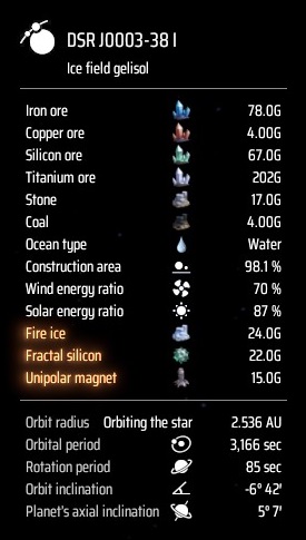
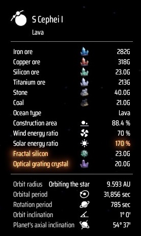It should be noted that actual efficiency of solar panels on the lava planet is ‘only’ 1.95 times as efficient as the one on the ice giant. Why the part ‘only’? One of those planets is around an O class blue giant, with luminosity of 2.413

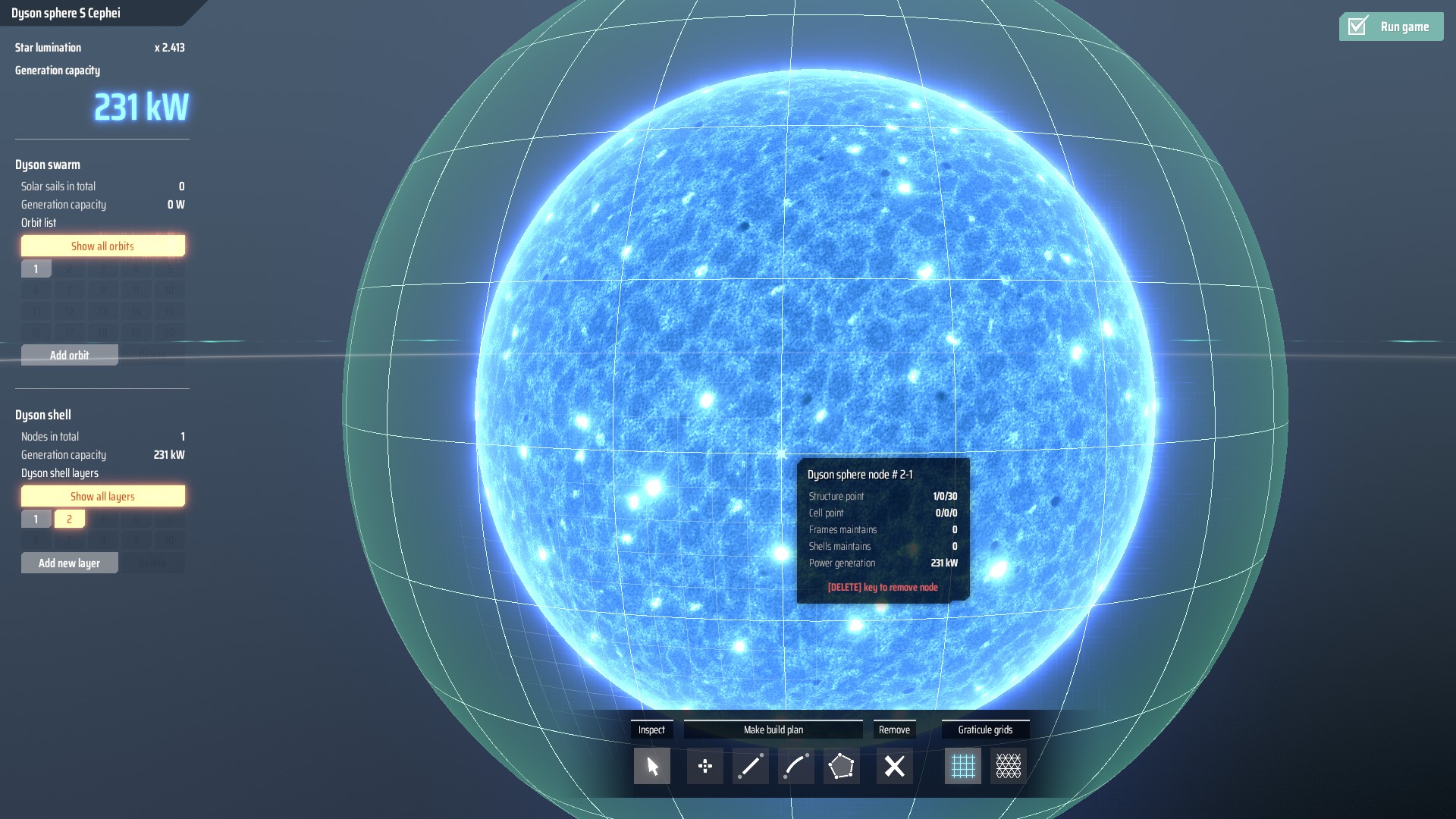
The other is around X class star… or rather remnants of a star – a black hole with luminosity of 0.177

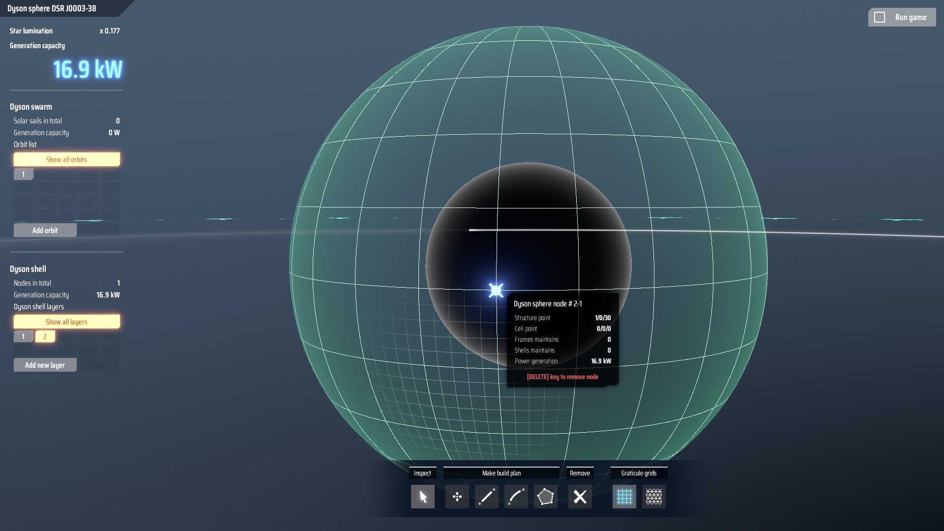
The difference in production of a Dyson system between the two is [as seen above] that blue giant star Dyson will produce 13.6 times as much energy per structure/cell point as one above the black hole.

This leads to quite easy note: Dyson cell points will be more cost-efficient on high luminosity stars with low solar performance modifier on planets, while solar panels will be way more cost efficient on low luminosity stars/planets with high solar power production modifier, and if we go by the cost of iron, we will want the luminosity to be 2x or higher the power modifier on the planet. Which admittedly is not that common [ note: Our ‘local’ value of resources may differ due to accessibility of silicon/copper/iron and stone].

As a side note – solar power modifier has lower variance than luminosity of stars.

Sooo… grab solar panels and be done with it as better/cheaper most of the time?
Here is where it becomes a bit more interesting.
At the start I made a claim that both solar and Dyson have their uses; What Dyson loses on cost efficiency [which frankly is not surprising in the least] it makes up in power density [again].

It takes from 13.8 solar panels [at minimum continuous running] to 34.7 [at maximum continuous running], at solar power modifier 100% to match power retrieval from a single receiver… using default settings. With graviton lens and photon method [at the cost of non-renewable resources] that amount increases to approx 361.1 solar panels to match energy output of a single receiver. In the case where tidal locked planet is available – standard receivers will be able to reclaim much higher amounts of energy than solar panels ever could, simply due to space efficiency. Though it should be taken into account that solar panels are much smaller structures.

To put it into perspective; at planet with 100% solar energy modifier, both solar panels and receiver will generate roughly the same amount of energy [with a minor UNDERPRODUCTION on the solar panel side, but below 1 solar panel], at the beginning of a period of energy receiving: [0% continuous receiving modifier from receiver].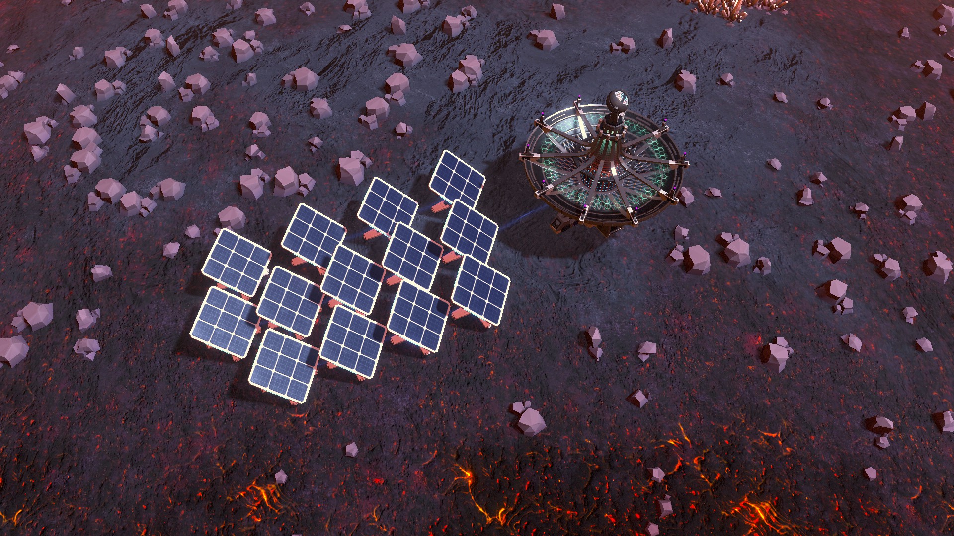

At 100% continuous receiving modifier you will need more solar panels to match a single receiver:

And that’s comparison WITHOUT any graviton lensing or photon processing method in the first place.

Additionally – solar panels work from solar energy [duh], and require direct line of sight to the star itself [even if the star is covered by Dyson sphere it has no impact on LOS detection of the star, due to lack of occlusion mechanics]. Receivers need direct line of sight to the Dyson System, which always is bigger than the star [by the very nature of the system], greatly increasing the area on which receivers can accept power, and can be used to power the grid. As an additional note – it should be restated that receivers do not care about amount of sunlight they receive, they only care about duration of connection [which admittedly rises more slowly, and drops instantly, but is not dependent on day cycle of the planet].

This in turn makes solar panels cost efficient for small scale, but have lower ability to scale up, and are much less space-efficient than receivers.

Afterword

As this data was obtained in experimental mode, not every mechanics and trick is known to me, and I am but a human.

If any of commentators finds any error or mistake please let me know, I will gladly fix it.

If you have any idea for improvement of this guide please let me know.

I would like to thank ampersin for feedback via discord, on improvements to the guide.

I would like to thank donschmiddy, for his attempt to optimize the power efficiency designs, and his insight into mathematical aspects of optimization.

I would like to thank Alavaria for her notice of node integration mechanics implications, and method to reduce amount of resources required for integration of shells.

Addendum:
Please keep in mind that if comments are not civil [insults, slurs, etc.] OR are intended as a business opportunity [a.k.a. ‘do this and I’ll do that in exchange], or are of spam nature [advertising, also – as above] they WILL be removed.
This is note added after an ‘exchange’ type comment was added as a comment to this guide.